“Open source software is software that can be freely accessed, used, changed, and shared (in modified or unmodified form) by anyone” (cp. https://opensource.org/osd). So open source software (OSS) is actually something that one or more people can work on, improve it, refine it, change it, adapt it and share or use it. Why would anyone support such a feature? Examples from the industry show that this is a valid approach for many software products. Prominent open source projects are in use worldwide on an everyday basis, including the Apache Web Server, the Linux Kernel, the GNU Compiler Collection, Samba, OpenSSL, and MySQL. For industry this means not only re-using components, and libraries, but also being able to fix them, adapt them to their needs and hire people who are already familiar with the tools. Business models based on open source software focus more on services than products and ensure the longevity of the software as even if companies vanish, the open source software is here to stay.
In academia open source provides a way to employ well-known methods as a base line or a starting point without having to re-invent the wheel by programming algorithms and methods all over again. This is especially popular in multimedia research, which would not be as agile and forward looking if it weren’t for OpenCV, ffmpeg, Caffe, and SciPy and NumPy, just to name a few. In research the need for publishing source code and data along with the scientific publication to ensure reproducibility has been identified recently (cp. ACM Artifact Review and Badging, https://www.acm.org/publications/policies/artifact-review-badging). This of course includes stronger support for releasing software and data artifacts based on open licenses.
The SIGMM community has been very active in this regard, since ACM Intl. Conference on Multimedia hosts the Open Source Software Competition since 2004; this competition has attracted in the latest years an increasing number of submissions and, according to Google Scholar, two of the currently three top cited papers in the last 5 years of the conference were submitted to this competition. This year also the ACM Intl. Conference on Multimedia Retrieval has introduced an OSS track.
Our aim for SIGMM Records is to point out recent development, announce interesting releases, share insights from the community and actively support knowledge transfer from research to industry based on open source software and open data four times a year. If you are interested in writing for the open source column, or have something you would like to know more about in this area, please do not hesitate to contact the editors. Examples are articles on open source frameworks or projects like the Menpo project, the Siva Suite, or the Yael library.
The SIGMM Records editors responsible for the open source are dedicated to the cause and have quite some history with open source in academia and industry.
Marco Bertini (https://github.com/mbertini) is associate professor at the University of Florence and long term open source supporter, especially by having served as chair and co-chair of the open source software competition at ACM Intl. Conference on Multimedia.
Mathias Lux (https://github.com/dermotte) has participated in the very same challenge with several open source projects. He’s associate professor at Klagenfurt University and dedicated to open source in research and teaching and main contributor to several open source projects.
The Menpo Project [1] is a BSD-licensed set of tools and software designed to provide an end-to-end pipeline for collection and annotation of image and 3D mesh data. In particular, the Menpo Project provides tools for annotating images and meshes with a sparse set of fiducial markers that we refer to as landmarks. For example, Figure 1 shows an example of a face image that has been annotated with 68 2D landmarks. These landmarks are useful in a variety of areas in Computer Vision and Machine Learning including object detection, deformable modelling and tracking. The Menpo Project aims to enable researchers, practitioners and students to easily annotate new data sources and to investigate existing datasets. Of most interest to the Computer Vision is the fact that The Menpo Project contains completely open source implementations of a number of state-of-the-art algorithms for face detection and deformable model building.
Figure 1. A facial image annotated wih 68 sparse landmarks.
In the Menpo Project, we are actively developing and contributing to the state-of-the-art in deformable modelling[2], [3], [4], [5]. Characteristic examples of widely used state-of-the-art deformable model algorithms are Active Appearance Models[6],[7], Constrained Local Models[8], [9] and Supervised Descent Method[10]. However, there is still a noteworthy lack of high quality open source software in this area. Most existing packages are encrypted, compiled, non-maintained, partly documented, badly structured or difficult to modify. This makes them unsuitable for adoption in cutting edge scientific research. Consequently, research becomes even more difficult since performing a fair comparison between existing methods is, in most cases, infeasible. For this reason, we believe the Menpo Project represents an important contribution towards open science in the area of deformable modelling. We also believe it is important for deformable modelling to move beyond the established area of facial annotations and to extend to a wide variety of deformable object classes. We hope Menpo can accelerate this progress by providing all of our tools completely free and permissively licensed.
Project Structure
The core functionality provided by the Menpo Project revolves around a powerful and flexible cross-platform framework written in Python. This framework has a number of subpackages, all of which rely on a core package called menpo. The specialised subpackages are all based on top of menpo and provide state-of-the-art Computer Vision algorithms in a variety of areas (menpofit, menpodetect, menpo3d, menpowidgets).
menpo – This is a general purpose package that is designed from the ground up to make importing, manipulating and visualising image and mesh data as simple as possible. In particular, we focus on data that has been annotated with a set of sparse landmarks. This form of data is common within the fields of Machine Learning and Computer Vision and is a prerequisite for constructing deformable models. All menpo core types are Landmarkable and visualising these landmarks is a primary concern of the menpo library. Since landmarks are first class citizens within menpo, it makes tasks like masking images, cropping images within the bounds of a set of landmarks, spatially transforming landmarks, extracting patches around landmarks and aligning images simple. The menpo package has been downloaded more than 3000 times and we believe it is useful to a broad range of computer scientists.
menpofit – This package provides all the necessary tools for training and fitting a large variety of state-of-the-art deformable models under a unified framework. The methods can be roughly split in three categories:
Generative Models: This category includes implementations of all variants of the Lucas-Kanade alignment algorithm [6], [11], [2], Active Appearance Models [7], [12], [13], [2], [3] and other generative models [14], [4], [5].
Discriminative Models: The models of this category are Constrained Local Models [8] and other closely related techniques [9].
Regression-based Techniques: This category includes the commonly-used Supervised Descent Method [10] and other state-of-the-art techniques [15], [16], [17].
The menpofit package has been downloaded more than 1000 times.
menpodetect – This package contains methodologies for performing generic object detection in terms of a bounding box. Herein, we do not attempt to implement novel techniques, but instead wrap existing projects so that they integrate natively with menpo. The current wrapped libraries are DLib, OpenCV, Pico and ffld2.
menpo3d – Provides useful tools for importing, visualising and transforming 3D data. menpo3d also provides a simple OpenGL rasteriser for generating depth maps from mesh data.
menpowidgets – Package that includes Jupyter widgets for ‘fancy’ visualization of menpo objects. It provides user friendly, aesthetically pleasing, interactive widgets for visualising images, pointclouds, landmarks, trained models and fitting results.
The Menpo Project is primarily written in Python. The use of Python was motivated by its free availability on all platforms, unlike its major competitor in Computer Vision, Matlab. We believe this is important for reproducible open science. Python provides a flexible environment for performing research, and recent innovations such as the Jupyter notebook have made it incredibly simple to provide documentation via examples. The vast majority of the execution time in Menpo is actually spent in highly efficient numerical libraries and bespoke C++ code, allowing us to achieve sufficient performance for real time facial point tracking whilst not compromising on the flexibility that the Menpo Project offers.
Note the Menpo Project has benefited enormously from the wealth of scientific software available with the Python ecosystem! The Menpo Project borrows from the best of the scientific software community wherever possible (e.g. scikit-learn, matplotlib, scikit-image, PIL, VLFeat, Conda) and the Menpo team have contributed patches back to many of these projects.
Getting Started
We, as the Menpo team, are firm believers in making installation as simple as possible. The Menpo Project is designed to provide a suite of tools to solve a complex problem and therefore has a complex set of 3rd party library dependencies. The default Python packing environment does not make this an easy task. Therefore, we evangelise the use of the Conda ecosystem. In our website, we provide detailed step-by-step instructions on how to install Conda and then Menpo on all platforms (Windows, OS X, Linux) (please see http://www.menpo.org/installation/). Once the conda environment has been set up, installing each of the various Menpo libraries can be done with a single command, as:
As part of the project, we maintain a set of Jupyter notebooks that help illustrate how Menpo should be used. The notebooks for each of the core Menpo libraries are kept inside their own repositories on our Github page, i.e. menpo/menpo-notebooks, menpo/menpofit-notebooks and menpo/menpo3d-notebooks. If you wish to view the static output of the notebooks, feel free to browse them online following these links: menpo, menpofit and menpo3d. This gives a great way to passively read the notebooks without needing a full Python environment. Note that these copies of the notebook are tied to the latest development release of our packages and contain only static output and thus cannot be run directly – to execute them you need to download them, install Menpo, and open the notebook in Jupyter.
Usage Example
Let us present a simple example that illustrates how easy it is to manipulate data and train deformable models using Menpo. In this example, we use annotated data to train an Active Appearance Model (AAM) for faces. This procedure involves four steps:
Loading annotated training images
Training a model
Selecting a fitting algorithm
Fitting the model to a test image
Firstly, we will load a set of images along with their annotations and visualize them using a widget. In order to save memory, we will crop the images and convert them to greyscale. For an example set of images, feel free to download the images and annotatons provided by [18] from here. Assuming that all the image and PTS annotation files are located in /path/to/images, this can be easily done as:
import menpo.io as mio
from menpowidgets import visualize_images

images = []
for i in mio.import_images('/path/to/images', verbose=True):
    i = i.crop_to_landmarks_proportion(0.1)
    if i.n_channels == 3:
        i = i.as_greyscale()
    images.append(i)

visualize_images(images) # widget for visualising the images and their landmarks
An example of the visualize_images widget is shown in Figure 2.
Figure 2. Visualising images inside Menpo is highly customizable (within a Jupyter notebook)
The second step involves training the Active Appearance Model (AAM) and visualising using an interactive widget. Note that we use Image Gradients Orientations [13], [11] features to help improve the performance of the generic AAM we are constructing. An example of the output of the widget is shown in Figure 3.
from menpofit.aam import HolisticAAM
from menpo.feature import igo

aam = HolisticAAM(images, holistic_features=igo, verbose=True)

print(aam) # print information regarding the model
aam.view_aam_widget() # visualize aam with an interactive widget
Figure 3. Many of the base Menpo classes provide visualisation widgets that allow simple data exploration of the created models. For example, this widget shows the joint texture and shape model of the previously created AAM.
Next, we need to create a Fitter object for which we specify the Lucas-Kanade algorithm to be used, as well as the number of shape and appearance PCA components.
from menpofit.aam import LucasKanadeAAMFitter

fitter = LucasKanadeAAMFitter(aam, n_shape=[5, 15], n_appearance=0.6)
Assuming that we have a test_image and an initial bounding_box, the fitting can be executed and visualized with a simple command as:
from menpowidgets import visualize_fitting_result

fitting_result = fitter.fit_from_bb(test_image, bounding_box)
visualize_fitting_result(fitting_result) # interactive widget to inspect a fitting result
An example of the visualize_fitting_result widget is shown in Figure 4.
Now we are ready to fit the AAM to a set of test_images. The fitting process needs to be initialized with a bounding box, which we retrieve using the DLib face detector that is provided by menpodetect. Assuming that we have imported the test_images in the same way as shown in the first step, the fitting is as simple as:
from menpodetect import load_dlib_frontal_face_detector

detector = load_dlib_frontal_face_detector() # load face detector

fitting_resutls = []
for i, img in enumerate(test_images):
    # detect face's bounding box(es)
    bboxes = detector(img)

    # if at least one bbox is returned
    if bboxes:
        # groundtruth shape is ONLY useful for error calculation
        groundtruth_shape = img.landmarks['PTS'].lms
        # fit
        fitting_result = fitter.fit_from_bb(img, bounding_box=bboxes[0],
                                            gt_shape=groundtruth_shape)
        fitting_resutls.append(fitting_result)

visualize_fitting_result(fitting_results) # visualize all fitting results
Figure 4. Once fitting is complete, Menpo provides a customizable widget that shows the progress of fitting a particular image.
landmarker.io is a web application for annotating 2D and 3D data, initially developed by the Menpo Team and then heavily modernised by Charles Lirsac. It has no dependencies beyond a modern web browser and is designed to be simple and intuitive to use. It has several exciting features such as Dropbox support, snap mode (Figure 6) and easy integration with the core types provided by the Menpo Project. Apart from the Dropbox mode, it also supports a server mode, in which the annotations and assets themselves are served to the client from a separate server component which is run by the user. This allows researches to benefit from the web-based nature of the tool without having to compromise privacy or security. The server utilises Menpo to import assets and save out annotations. An example screenshot is given in Figure 5.
The application is designed in such a way to allow for efficient manual annotation. The user can also annotate any object class and define their own template of landmark labels. Most importantly, the decentralisation of the landmarking software means that researchers can recruit annotators by simply directing them to the website. We strongly believe that this is a great advantage that can aid towards acquiring large databases of correctly annotated images for various object classes. In the near future, the tool will support a semi-assisted annotation procedure, for which Menpo will be used to provide initial estimations of the correct points for the images and meshes of interest.
Figure 5. The landmarker provides a number of methods of importing assets, including from Dropbox and a custom Menpo server.
Figure 6. The landmarker provides an intuitive snap mode that enables the user to efficiently edit a set of existing landmarks.
[/caption]
Conclusion and Future Work
The research field of rigid and non-rigid object alignment lacks of high-quality open source software packages. Most researchers release code that is not easily re-usable, which further makes it difficult to compare existing techniques in a fair and unified way. Menpo aims to fill this gap and give solutions to these problems. We put a lot of effort on making Menpo a solid platform from which researchers of any level can benefit. Note that Menpo is a rapidly changing set of software packages that attempts to keep track of the recent advances in the field. In the future, we aim to add even more state-of-the-art techniques and increase our support for 3D deformable models [19]. Finally, we plan to develop a separate benchmark package that will standarize the way comparisons between various methods are performed.
Note that by the time this article was released, the versions of the Menpo packages were as follows:
If you have any questions regarding Menpo, please let us know on the menpo-users mailing list.
References
[1] J. Alabort-i-Medina, E. Antonakos, J. Booth, P. Snape, and S. Zafeiriou, “Menpo: A comprehensive platform for parametric image alignment and visual deformable models,” in Proceedings Of The ACM International Conference On Multimedia, 2014, pp. 679–682. http://doi.acm.org/10.1145/2647868.2654890
[2] E. Antonakos, J. Alabort-i-Medina, G. Tzimiropoulos, and S. Zafeiriou, “Feature-based lucas-kanade and active appearance models,” Image Processing, IEEE Transactions on, 2015. http://dx.doi.org/10.1109/TIP.2015.2431445
[3] J. Alabort-i-Medina and S. Zafeiriou, “Bayesian active appearance models,” in Computer Vision And Pattern Recognition (CVPR), 2014 IEEE Conference On, 2014, pp. 3438–3445. http://dx.doi.org/10.1109/CVPR.2014.439
[6] S. Baker and I. Matthews, “Lucas-kanade 20 years on: A unifying framework,” International Journal of Computer Vision, vol. 56, no. 3, pp. 221–255, 2004. http://dx.doi.org/10.1023/B:VISI.0000011205.11775.fd
[8] J. M. Saragih, S. Lucey, and J. F. Cohn, “Deformable model fitting by regularized landmark mean-shift,” International Journal of Computer Vision, vol. 91, no. 2, pp. 200–215, 2011. http://dx.doi.org/10.1007/s11263-010-0380-4
[9] A. Asthana, S. Zafeiriou, G. Tzimiropoulos, S. Cheng, and M. Pantic, “From pixels to response maps: Discriminative image filtering for face alignment in the wild,” 2015. http://dx.doi.org/10.1109/TPAMI.2014.2362142
[10] X. Xiong and F. De la Torre, “Supervised descent method and its applications to face alignment,” in Computer Vision And Pattern Recognition (CVPR), 2013 IEEE Conference On, 2013, pp. 532–539. http://dx.doi.org/10.1109/CVPR.2013.75
[11] G. Tzimiropoulos, S. Zafeiriou, and M. Pantic, “Robust and efficient parametric face alignment,” in Computer Vision (ICCV), 2011 IEEE International Conference On, 2011, pp. 1847–1854. http://dx.doi.org/10.1109/ICCV.2011.6126452
[12] G. Papandreou and P. Maragos, “Adaptive and constrained algorithms for inverse compositional active appearance model fitting,” in Computer Vision And Pattern Recognition (CVPR), 2008 IEEE Conference On, 2008, pp. 1–8. http://dx.doi.org/10.1109/CVPR.2008.4587540
[13] G. Tzimiropoulos, J. Alabort-i-Medina, S. Zafeiriou, and M. Pantic, “Active orientation models for face alignment in-the-wild,” Information Forensics and Security, IEEE Transactions on, vol. 9, no. 12, pp. 2024–2034, 2014. http://dx.doi.org/10.1109/TIFS.2014.2361018
[14] G. Tzimiropoulos and M. Pantic, “Gauss-newton deformable part models for face alignment in-the-wild,” in Computer Vision And Pattern Recognition (CVPR), 2014 IEEE Conference On, 2014, pp. 1851–1858. http://dx.doi.org/10.1109/CVPR.2014.239
[15] A. Asthana, S. Zafeiriou, S. Cheng, and M. Pantic, “Incremental face alignment in the wild,” in Computer Vision And Pattern Recognition (CVPR), 2014 IEEE Conference On, 2014, pp. 1859–1866. http://dx.doi.org/10.1109/CVPR.2014.240
[16] V. Kazemi and J. Sullivan, “One millisecond face alignment with an ensemble of regression trees,” in Computer Vision And Pattern Recognition (CVPR), 2014 IEEE Conference On, 2014, pp. 1867–1874. http://dx.doi.org/10.1109/CVPR.2014.241
[19] V. Blanz and T. Vetter, “A morphable model for the synthesis of 3D faces,” in Proceedings Of The 26th Annual Conference On Computer Graphics And Interactive Techniques, 1999, pp. 187–194. http://dx.doi.org/10.1145/311535.311556
Alphabetical author order signifies equal contribution↩
Currently unreleased – the next released versions of menpo, menpofit and menpodetect will reflect these version numbers. All samples were written using the current development versions.↩
The SIVA Suite is an open source framework for the creation, playback, and administration of hypervideos. Allowing the definition of complex navigational structures, our hypervideos are well suited for different scenarios. Compared to traditional linear videos, they especially excel in e-learning and training situations (see [1] and [2]), where fitting the teaching material to the needs of the viewer can be crucial. Other fields of application include virtual tours through buildings or cities, sports events, and interactive video stories. The SIVA Suite consists of an authoring tool (SIVA Producer), an HTML5 hypervideo player (SIVA Player), and a Web server (SIVA Server) for user and video management. It has been evaluated in various scenarios with several usability tests and has been improved step-by-step since 2008.
Introduction
The viewer of a traditional video takes a mostly passive role. Traditional videos are linear and cannot provide additional information about objects or scenes. In contrast to traditional linear videos, hypervideos are not only made of a sequence of video scenes. Their essence are alternative storylines, user choices, and additional materials which can be viewed in parallel with the main content as well as a navigational structure facilitating these features. Therefore, special players with extended controls and areas to present the additional information beyond the original content are necessary. The user choices in the video can be made at the selection of the follow-up scene on a button panel, a table of contents, as well as a keyword search.
One of the most advanced tools in this area is Hyper-Hitchcock [3] which can be used for the creation of detail-on-demand hypervideos with one main storyline and entry points for more detailed video explanations. However, an open source version of the software is not available. With new technologies like HTML5, CSS 3, and JavaScript, web-based tools like Klynt [4] emerged. Klynt allows the creation of hypervideos with focus on different media types and provides many useful features but can not be extended or customized due to the proprietary licensing. Finally, with the SIVA Suite we now offer the first customizable open source framework for the creation of hypervideos.
To simplify the creation process, our work focuses on videos as the main content. In the SIVA Producer, video scenes and navigational elements are arranged in a graph, called scene graph, to define the navigational structure of a hypervideo. Annotations offering additional information can be added to single scenes as well as to the whole video. For this purpose, images, texts, pdfs, audios, and even videos may be used. As a supplement to the video structure defined by the scene graph, further navigational elements like a table of contents and a keyword search enable the viewer to easily jump to points of interest.
Hypervideos are created in the SIVA Producer and then uploaded to the SIVA Server. Registered users can then download the video from the server or watch it online. If logging is enabled, user interactions during playback are logged by the player and sent to the database on the SIVA Server. Video administrators can access the logging data and watch different diagrams or export the data for further analysis in a statistics tool. An overview of the system is shown in Figure 1.
The SIVA Producer is used for the creation of hypervideos where main video scenes are linked with each other in a scene graph. Each of the scenes may have one or more multimedia annotations. Further navigational structures are a table of contents as well as the definition of keywords which can then be searched for in the player. The GUI was implemented and improved step-by-step since 2008 [5]
First Steps
Create a new project: A new project is created with a wizard. The author can set the appearance of the player as well as functions the player will provide. It is, for example, possible to select a primary and a secondary color, to determine the width of the annotation panel, etc.
Add media files to the project: Media files are imported into the media repository. These may be videos, audios, images, or html files. The Producer uses each media file in its original format during the creation process and only transforms it during the export.
Create scenes: From videos in the media repository, scenes can be extracted. Those will be added to the scene repository from where they can be dragged to the scene graph to create the hypervideo structure.
Create a scene graph: A scene graph (see Figure 2) consists of a defined start and an end, as well as several scenes and connection/branching elements allowing advanced navigation options during playback of the video. Scenes and navigation elements are added to the scene graph via drag and drop. These elements are linked with the connection tool from the scene graph tool bar. In order to produce a valid and exportable scene graph, two conditions have to be met. First, only one start scene is allowed. Second, every scene has to be connected by some path to the start and to the end of the video. The validity of the scene graph can be checked with a validation function.
Figure 2. Scene graph of the SIVA Producer.
Add annotations to scenes: Each scene in the scene graph may have one or more multimedia annotations. To add an annotation, a media file can either be dragged from the media repository and dropped on a scene, or an annotation editor (see Figure 3) can be used to customize its timing and appearance. Additionally, a hotspot can be added to the scene which invokes the display of the annotation only after a viewer clicks the marked area.
Figure 3. Annotation editor of the SIVA Producer.
Export video project: In a last step, finished hypervideo projects with valid scene graphs are exported for the player. The structure of the hypervideo with all possible actions is converted into a JSON file. The media files are transformed and transcoded for the desired target platform.
Further Features
Global annotations: Besides annotations which are displayed with scenes, global annotations which are displayed during the whole hypervideo (and do not have timing information as a consequence) can be added with a separate editor. The editor is opened from the main menu or the quick access toolbar.
Keywords: Keywords can be added to scenes and annotations in the respective editors. They are added in whitespace-separated lists at the lower left part of the editors. Currently, only keywords added by the author are exported to the player and searchable with the search function, no automated analysis of the media files is performed.
Table of contents: The table of contents editor (see Figure 4) is used to create a tree structure of entries with meaningful headlines. A scene from the scene graph can be linked with one of the entries in the table of contents. A scene is added to an entry in the table of contents via drag and drop. The editor is opened from the main menu or the quick access toolbar.
Figure 4. Table of contents editor of the SIVA Producer.
Advanced navigation: Besides a standard selection element where the user may select one of the attached paths to continue playback in the player, more advanced elements are available as well:
Forward button: A single button with only one label. It can be used to interrupt a linear sequence of scenes.
Random selection: One of the attached paths will be selected at random without user interaction.
Conditional selection: For attached paths, conditions can be defined which have to be fulfilled before the path is unlocked for playback.
Project handover: The SIVA Producer provides a function for handing over a project to another computer. Using this function, all media files as well as the project file are copied into a given file structure where they can easily be copied from.
Help: A help for the SIVA Producer can be found in the menu under “Help -> Help Contents“.
SIVA Player
Reqirements (recommended):
Firefox 42.0, Chrome 46.0, Opera 33, Internet Explorer 11, Safari 10.10
Installation:
use HTML export profile in SIVA Producer, then integrate it into a website via copying the body part of the exported HTML file and adapting the paths – or use as local stand-alone player
The SIVA Player is used to play the hypervideo created in the SIVA Producer. The structure and media elements of the hypervideo are described in a JSON file which conforms to the XML structure described in [6]. A previous versions of the player can be found in [7].
Figure 5. SIVA Player with video view and annotation area.
The playback of the described videos requires special players which are capable of providing navigational elements like selection panels for follow-up scenes, a table of contents, or a search function. Furthermore, areas for displaying additional information are necessary. Figure 5 shows a user interface of the player (with contents of a medical training scenario) with the following elements:
(1) standard controls like pause/play
(2) a progress bar (for the current video)
(3) a settings button
(4) a volume control
(5) entry point to the table of contents
(6) a button to jump to the previous scene
(7) title of the currently displayed scene
(8) a button to jump to the next scene (or to a selection panel)
(9) a search button (performs a live search and refines the search results with every keystroke)
(10) a button for the full-screen mode
(11) a foldout panel on the right shows additional information (here, an additional video (12) and two image galleries (13); the additional video provides standard controls and can be displayed in full-screen mode (14))
A click on one of the annotations opens its contents in full screen mode for additional interactions (like browsing an image gallery or watching a video), while the player pauses the main video in the background. If a fork is reached in the scene graph, a button panel is provided at the left side of the main video area where the viewer has to select the next scene. The player also provides multiple language support if the author provides translations for all text and media elements (note: this functionality is not yet implemented in the SIVA Producer, the translations have to be made manually in the JSON file). Besides clicking or tapping the buttons, the basic functions of the player can also be controlled using the keyboard, namely with space bar, ESC button, and left and right arrow button.
All actions of the user can be recorded if logging is enabled by the author. The player transmits the actions to the server every 60 seconds as well as when the player starts or the video ends, if it is used in online mode. If the player is used in offline mode, logging data is collected and transmitted to the server when a connection can be established.
Configurations in HTML are possible. Using a responsive design, the player cannot only be used on desktop PCs having varying screen sizes but also on mobile devices in landscape and portrait mode. The player can be used online over the internet or in offline mode when all files are stored at the end user device.
The SIVA Server provides a platform for hypervideos and evaluations based on logging data. Furthermore, it provides user and rights management for copyright protected videos.
Videos exported by the producer are uploaded in the Web interface, extracted by the server, and can then be viewed on the server. It is furthermore possible to provide a link to a video, for example when the video is also available as a Chrome App, or a download for a zip file. The latter can be extracted locally on the end user device and watched without internet connection.
Users may have different roles (like user, administrator, etc.) and rights according to their roles. Furthermore, each user may be member of one or more groups. The accessibility of videos can be assigned at group level. This ensures that the visibility of videos is satisfied according to the demands of the author or copyright limitations. A help for the SIVA Server can be found on its start page.
Figure 6. SIVA Server – player stats with usage view.
The server furthermore provides the SIVA Player Stats, the back end for the logging functionality of the player. This part of the application facilitates analyzing and evaluating the logged usage data. Watching, searching, exporting, or visualizing these data can be done video based. One of the currently available diagram views is the Sunburst diagram (see Figure 6), which shows how often certain paths were taken in a video by the viewers. Another diagram is a Treemap which shows the different scenes of the video and the events in these scenes. Thereby, the sizes of the boxes are representing the frequency of occurrence of one single event. This part of the application is only accessible for administrators registered in the front-end.
In this column we present the SIVA Suite, an open source framework for the creation, playback, and administration of hypervideos. The authoring tool, the SIVA Producer, provides several editors like a scene graph or annotation editors, as well as an export function. The hypervideo player, the SIVA Player, has extended controls and display areas as well as an intuitive design. The Web server, the SIVA Server, provides functions for user, group, and video management. This framework, especially the authoring tool and the player, were successfully used for the creation and playback of several hypervideos, most noteworthy a medical hypervideo training (see [1] and [2]). Both were evaluated in several usability tests and improved step-by-step since 2008.
While the framework already provides all necessary functions for the creation, playback, and management of hypervideos, several additional functions might be desirable. For now, video conversion is done in the producer during the export of a hypervideo. Especially when several video versions (regarding resolution, quality, or video format) are needed, this task can block the production site for a long period. To improve productivity, video conversion could be moved to the server component. Furthermore, a player preview in the producer is preferable, which avoids the necessity to export the hypervideo to watch it. While currently a created hypervideo can only be translated by manually copying its structure to a new project, input forms for multilingualism in the producer would make this task easier. Pushing the interaction part to a new level, viewers could benefit from a collaborative editing function in the player, allowing them to add comments or additional materials to a video. Additionally, splitting the contents of the player into a second screen could allow for easier interaction and perception of hypervideos, especially in sports or medical training scenarios. The implementation of a download and cache management as described in [9] and [10] in the player may help to reduce waiting time at scene changes.
[2] Britta Meixner, Katrin Tonndorf, Stefan John, Christian Handschigl, Kai Hofmann, Michael Granitzer, Michael Langbauer & Harald Kosch. A Multimedia Help System for a Medical Scenario in a Rehabilitation Clinic. In: Proceedings of I-Know, 14th International Conference on Knowledge Management and Knowledge Technologies (i-KNOW ’14). ACM, New York, NY, USA, 25:1-25:8, 2014.
The program of ACM Multimedia is very diverse: apart from oral and poster presentations, panels and keynotes there are challenges and competitions. One that is particularly interesting is the Open Source Software Competition, which is pretty much specific for this conference and was started in ACM Multimedia 2004. The full list of participants and winners (along with links to all the projects) can be found on the SIGMM web site: http://sigmm.org/Resources/software/ossc. This list shows that over the years this session has drawn a larger (and well deserved) attention from the community. We have asked the chairs of the ACM MM 2013 (Andrea Vedaldi & Ioannis Patras, answering as Org2013) and 2015 (Xian-Sheng Hua, Marco Bertini & Tao Mei, answering as Org2015) competition about their experience and opinions about the competition.
Q1: How hard was to get submissions to OSSC? Did you have to ask authors of software you knew or are they aware of this part of the ACM MM programme? Overall how many submissions did you receive?
Org2013: We did not have to ask any author directly. We only circulated an advertisement to three mailing lists, including a CV and ML one. The competition seems to be sufficiently well known that it is capable to attract submission with little effort.
Org2015: It was not that hard, we contacted some authors asking for submissions, but in the end the majority of submissions came from people who already knew the competition or from the call for paper we disseminated. We received 15 submissions, of which 9 were accepted. Decisions were taken considering the quality of the presentation and of the software itself, as well as the importance and utility for the multimedia community.
Q2: What’s your evaluation of the quality of submissions? Have you ever used software from past submissions?
Org2013: Half of the submission were of very high quality, both in scope and maturity of the projects. A few very very poor, at the level of master project at most. (Note: Andrea won the ACM MM’10 competition with his VLFeat library).
Org2015: Quality is quite high, we accepted works that were interesting and useful for the community and that were also mature enough to be used by members of the multimedia community. Marco Bertini: I already use some software of the submissions of this year, and I am using also software from past editions.
Q3: What’s your evaluation of OSSC per-se? Do you think other conferences should have something similar?
Org2013: It is a very good competition as it gives a chance to the authors of the software to obtain a publication and significant publicity (especially in the case of victory). It is also a great way to let the public know about solid OS projects. Having multiple competitions is tempting as contributions tend to be quite orthogonal (e.g. audio vs database vs networking vs imaging). At the same time, the number of contributions does not seem to warrant splitting the effort up.
Org2015: It is an interesting and useful track for ACM Multimedia. It has both scientific and technical value: It eases the development of new algorithms and methods, and allows to re-implement more easily the methods proposed by other researchers. The effort of the authors of such software deserve to be recognized by the scientific community. Probably other major conferences in different fields of CS should introduce this type of track.
Yael is a library implementing computationally intensive functions used in large scale image retrieval, such as neighbor search, clustering and inverted files. The library offers interfaces for C, Python and Matlab.
The motivation of Yael is twofold. We aim at providing:
core and optimized instructions and methods commonly used for large-scale multimedia retrieval systems
more sophisticated functions associated with state-of-the-art methods, such as the Fisher vector, VLAD, Hamming Embedding or more generally methods based on inverted file systems, such as selective match kernels.
Yael is intended as an API and does not implement a retrieval system in an integrated manner: only a few test programs are available for key tasks such as k-means. Yet this can be done on top of it with a few dozen lines of Matlab or Python code.
Yael started as an open-source spin-off of INRIA LEAR‘s proprietary library Bigimbaz. The objective was to isolate performance-critical primitives that could be re-used in other projects. Yael’s design choices were: implemented in C for simplicity, but using an object-oriented design (structs with constructors/destructors), interface with Python as high-level language to facilitate administrative tasks.
Yael is designed to handle dense data in float, as it is primarily used for signal processing tasks where the quality of the representation is determined by the number of dimensions rather than the precision of the components. In the Matlab interface, single matrices, and float32 in Python. Yael was designed initially to manipulate matrices in C. It was interfaced for Python using SWIG, which gives low-level access to the full library. An additional Numpy layer (ynumpy) is provided for high-level functions. The most important functions of Yael are wrapped in Mex to be callable from Matlab.
Performance is very important. Yael has computed k-means with hundreds of thousand centroids and routinely manipulate matrices that occupy more than 1/2 the machine’s RAM. This means that it has to be lightweight and 64-bit clean. The design choices of Yael are governed by efficiency concerns more than by portability. As a result, the library may work only with severely down-graded performance if instructions are not provided by the processor. In particular, Yael relies on SSE instructions such as the SSE 4.2 popcnt instruction. The library is maintained for Linux and MacOS. Yael relies on as few external libraries as possible. The only mandatory ones are BLAS/Lapack (for performance). Other libraries (Python’s C interface, Matlab’s mex, Arpack, OpenMP) are optional.
Yael and related packages are downloaded around 600 times per month.
This article addresses the recognition of images of the same scene or object, and how Yael can perform this kind of operation. Here is an example of two images of the same scene that we would like to match:
We will explain how to compute descriptors (aka signatures) for the images, and how to find descriptors that are similar between images.
We are going to work on the 100 first query images of the Holidays dataset, and their associated database examples. The images and associated SIFT descriptors can be downloaded from here: Images and SIFT descriptors.
Image indexing
Imagine a user that has a large image collection with photos of buildings, with as associated metadata the GPS location of the building. Given a new photo of a building, taken with a mobile phone, the user wants to find the location where the photo was taken. This is where image indexing comes into play.
Image indexing means constructing an index referencing the images from a collection. This index has a search function that can be used to retrieve the images that are most similar to a query image.
At build time and search time, the index is stored in RAM. This is orders of magnitude faster than disk-based implementations, such as those used in SQL database engines. However, for large datasets, this requires either a lot of RAM or a very compact representation per image. Yael provides this compact representation, so that you do not need to buy the RAM.
In combination with efficient matrix manipulation environments like Matlab and Numpy, Yael makes the process of building an index and searching in it very simple.
Extracting image descriptors
Local image descriptors are vectors computed each on an area of the image. The areas are selected to contain strong contrast changes, with a 2D signal processing filter. Then the descriptor vector is computed from the gradient or frequency content in the area.
Local descriptors are typically designed to be invariant to some classes of transformations: translations, illumination changes, rotations, etc. At the same time, they should be discriminant enough to distinguish relevant differences on the patches, eg. different patterns on the facade of a building. There is a long line of research on designing local image features with appropriate tradeoffs in terms of invariance / discriminance / computational cost, see for example this comparison of affine covariant features.
In the images above, local descriptors extracted on the skyline ought to be very similar. Therefore, these images should be easy to match.
Local descriptors can be extracted using any local description algorithm, as long as they can be compared with L2 distances, ie. descriptors that are far away in L2 space are also considered different in image content. For example, OpenCV provides an implementation of the SURF descriptor, and VLFeat contains a SIFT implementation.
For this example, we will use the SIFT implementation provided along with the Holidays dataset. In the “Descriptor extraction” section of http://lear.inrialpes.fr/~jegou/data.php, download the executable (there is a Mac OS X version and a Linux version).
The pre-processing applied to images before analyzing them to extract signatures can have a dramatic effect on the retrieval performance. Ideally, images should be equalized so that their luminance is similar and resized into dimensions that are not too different. This can be performed in a number of ways, eg. with Imagemagick. In our case, we’ll just use a few command-line utilities from netpbm.
In total, the steps that extract the descriptors from a single image are:
This should be applied to all the images that are to be indexed, and the ones that will be queried.
The remainder of this article presents the main functions used in Yael to do image retrieval. They are implemented in the two languages supported by Yael: Python and Matlab.
Image indexing in Python with Fisher vectors
A global image descriptor is a vector that characterizes the whole image. The Euclidean distance between the descriptors of two images should be higher for different images than for similar images. There are many popular types of global descriptors, like color histograms or GIST descriptors.
The most important functions of Yael are available in Python via the ynumpy module. They all manipulate c-compact float32 or int32 matrices.
The FV computation relies on a training where a Gaussian Mixture Model (GMM) is fitted to a set of representative local descriptors. For simplicity, we are going to use the descriptors of the database we index. To load the database descriptors, use the ynumpy.siftgeo_read function:
for imname in image_names:
    desc, meta = ynumpy.siftgeo_read(imname)
    image_descs.append(desc)
The meta component contains the SIFT descriptor’s meta-information (location and size of the area, orientation, etc.). We do not use this information to compute the FV.
Next we sample the descriptors to reduce their dimensionality by PCA and computing a GMM. This involves some standard numpy code, and the ynumpy.gmm_learn function. For a GMM of size k (let’s set it to 64), we need about 1000*k training descriptors
k = 64
n_sample = k * 1000

# choose n_sample descriptors at random
sample_indices = np.random.choice(all_desc.shape[0], n_sample)
sample = all_desc[sample_indices]

# train GMM
gmm = ynumpy.gmm_learn(sample, k)
The GMM is a tuple containing the a-priori weights per mixture component, the mixture centres and the diagonal of the component covariance matrices (the model assumes a diagonal matrix, otherwise the descriptor would be way too long).
The training is finished. The next stage is to encode the SIFTs into one vector per image:
image_fvs = []
for image_desc in image_descs:
   # compute the Fisher vector, using only the derivative w.r.t mu
   fv = ynumpy.fisher(gmm, image_desc, include = 'mu')
   image_fvs.append(fv)
All the database descriptors are stacked as lines of a single matrix image_fvs, and all queries image descriptors in another matrix query_fvs. Then the Euclidean nearest neighbors of each query (and hence the most similar images) can be retrieved with:
# get the 8 NNs for all query images in the image_fvs array
results, distances = ynumpy.knn(query_fvs, image_fvs, nnn = 8)
Now we display the search results for a few query images. There is one line per query image, which shows the image, and a row of retrieval results. The correct results have a green rectangle around them, negative ones a red rectangle.
Note that the query image always appears as the first retrieval result, because it is included in the dataset.
Image indexing based on global descriptors like the Fisher Vector is very efficient and easy to implement using Yael. For larger datasets (more than a few tens of thousand images), it is useful to use vector quantization or hashing techniques to perform the nearest-neighbor search faster.
Image indexing in Matlab with inverted files
In this chapter, we directly index all the local SIFT descriptors of the database images into an indexing structure in RAM called the inverted file. Each SIFT descriptor is assigned an index in [1,k] using a quantization function. The inverted file contains k lists, one per possible index. When a SIFT from an image is assigned to an index 1 ≤ i ≤ k, the id of this image is added to the list i.
In the example below, we show how to use an inverted file of Yael from Matlab. More specifically, the inverted file we consider supports binary signatures, as proposed in the Hamming Embedding approach described in this paper.
Before launching the code, please ensure that
You have a working and compiled version of Yael’s matlab interface
The corresponding directory (‘YAELDIR/matlab’) is in your matlab Path. If not, use the addpath(‘YAELDIR/matlab’) to add it.
To start with, we define the parameters of the indexing method. Here, we choose a vocabulary of size k=1024. We also set some parameters specific to Hamming embedding.
k = 1024;                            % Vocabulary size
dir_data = './holidays_100/';        % data directory

% Parameters For Hamming Embedding
nbits = 128;                         % Typical values are 32, 64 or 128 bits
ht = floor(nbits*24/64);             % Hamming Embedding threshold
Hereafter, we show how we typically load a set of images and descriptors stored in separate files. We use the standard matlab functions arrayfun and cellfun to perform operations in batch. The descriptors are assumed stored in the siftgeo format, therefore we read them with the yael ‘siftgeo_read’ function.
sifts = cell();

for i = 1:numel(img_list)
  [sifts_i, meta] = siftgeo_read(img_list{i});
  sifts{i} = sifts_i;
end
Now, we are going to learn the visual vocabulary with k-means and subsequently construct the inverted file structure for Hamming Embedding. We learn it on Holidays itself to avoid requiring another dataset. But note that this should be avoided for a true system, and a proper evaluation should employ an external dataset for dictionary learning.
vtrain = [sifts{:}];
vtrain = vtrain (:, 1:2:end); tic

C = yael_kmeans (vtrain, k, 'niter', 10);

% We provide the codebook and the function that performs the assignment,
% here it is the exact nearest neighbor function yael_nn

ivfhe = yael_ivf_he (k, nbits, vtrain, @yael_nn, C);
We can add the descriptors of all the database images to the inverted file. Here, Each local descriptor receives an identifier. This is not a requirement: another possible choice would be to use directly the id of the image. But in this case we could not use this output for spatial verification. In our case, the descriptor id will be used to display the matches.
descid_to_imgid = zeros (totsifts, 1);  % desc to image conversion
imgid_to_descid = zeros (nimg, 1);      % for finding desc id
lastid = 0;

for i = 1:nimg
  ndes = nsifts(i);  % number of descriptors

  % Add the descriptors to the inverted file.
  % The function returns the visual words (and binary signatures),
  [vw,bits] = ivfhe.add (ivfhe, lastid+(1:ndes), sifts{i});
  imnorms(i) = norm(hist(vw,1:k));

  descid_to_imgid(lastid+(1:ndes)) = i;
  imgid_to_descid(i) = lastid;
  lastid = lastid + ndes;
end
Finally, we make some queries. We compute the number of matches n_immatches between query and database images. We invoke the standard Matlab function accumarray, which in essence compute here a histogram weighted by the match weights.
Queries = [1 13 23 42 63 83];
for q = 1:numel(Queries)
  qimg = Queries(q)

  matches = ivfhe.query (ivfhe, int32(1:nsifts(qimg)), sifts{qimg}, ht);

  % Translate to image identifiers and count number of matches per image,
  m_imids = descid_to_imgid(matches(2,:));
  n_immatches = hist (m_imids, 1:nimg);

  % Images are ordered by descreasing score
  [~, idx] = sort (n_immatches, 'descend');

  % Display results
  ...
end
The output looks as follows. The query is the top-left image, and then the queries are displayed. The title gives the number of matches and the normalized score used to rank the images. The matches are displayed in yellow (and the non-matching descriptors in red).
Conclusion
Yael is a small library that contains many primitives that are useful for image indexing, nearest-neighbor search, sorting, etc. It at the base of several state-of-the-art implementations of image indexing packages. Reference [1] describes the implementation tradeoffs of some of Yael’s main functions, and provides more references to research papers whose results were obtained with Yael.
In the code above, only the main function calls were shown, see the Yael tutorial for a fully functional version of the code, and the main Yael website for the complete documentation.
GamingAnywhere is an open-source clouding gaming platform. In addition to its openness, we design GamingAnywhere for high extensibility, portability, and reconfigurability. GamingAnywhere currently supports Windows and Linux, and can be ported to other OS’s including OS X and Android. Our performance study demonstrates that GamingAnywhere achieves high responsiveness and video quality yet imposes low network traffic [1,2]. The value of GamingAnywhere, however, is from its openness: researchers, service providers, and gamers may customize GamingAnywhere to meet their needs. This is not possible in other closed and proprietary cloud gaming platforms. A demonstration of the GamingAnywhere system. There are four devices in the photo. One game server (left-hand side labtop) and three game clients (an MacBook, an Android phone, and an iPad 2).
Motivation
Computer games have become very popular, e.g., gamers spent 24.75 billion USD on computer games, hardware, and accessories in 2011. Traditionally, computer games are delivered either in boxes or via Internet downloads. Gamers have to install the computer games on physical machines to play them. The installation process becomes extremely tedious because the games are too complicated and the computer hardware and system software are very fragmented. Take Blizzard’s Starcraft II as example, it may take more than an hour to install it on an i5 PC, and another hour to apply the online patches. Furthermore, gamers may find that their computers are not powerful enough to enable all the visual effects yet achieve high frame rates. Hence, gamers have to repeatedly upgrade their computers so as to play the latest computer games. Cloud gaming is a better way to deliver high-quality gaming experience and opens new business opportunities. In a cloud gaming system, computer games run on powerful cloud servers, while gamers interact with the games via networked thin clients. The thin clients are light-weight and can be ported to resource-constrained platforms, such as mobile devices and TV set-top boxes. With cloud gaming, gamers can play the latest computer gamers anywhere and anytime, while the game developers can optimize their games for a specific PC configuration. The huge potential of cloud gaming has been recognized by the game industry: (i) a market report predicts that cloud gaming market will increase 9 times between 2011 and 2017 and (ii) several cloud gaming startups were recently acquired by leading game developers. Although cloud gaming is a promising direction for the game industry, achieving good user experience without excessive hardware investment is a tough problem. This is because gamers are hard to please, as they concurrently demand for high responsiveness and high video quality, but do not want to pay too much. Therefore, service providers have to not only design the systems to meet the gamers’ needs but also take error resiliency, scalability, and resource allocation into considerations. This renders the design and implementation of cloud gaming systems extremely challenging. Indeed, while real-time video streaming seems to be a mature technology at first glance, cloud gaming systems have to execute games, handle user inputs, and perform rendering, capturing, encoding, packetizing, transmitting, decoding, and displaying in real-time, and thus are much more difficult to optimize. We observe that many systems researchers have new ideas to improve cloud gaming experience for gamers and reduce capital expenditure (CAPEX) and operational expenditure (OPEX) for service providers. However, all existing cloud gaming platforms are closed and proprietary, which prevent the researchers from testing their ideas on real cloud gaming systems. Therefore, the new ideas were either only tested using simulators/emulators, or, worse, never evaluated and published. Hence, very few new ideas on cloud gaming (in specific) or highly-interactive distributed systems (more general) have been transferred to the industry. To better bridge the multimedia research community and the game/software industry, we present GamingAnywhere, the first open source cloud gaming testbed in April 2013. We hope GamingAnywhere cloud gather enough attentions, and quickly grow into a community with critical mass, just like Openflow, which shares the same motivation with GamingAnywhere in a different research area.
Design Philosophy
GamingAnywhere aims to provide an open platform for researchers to develop and study real-time multimedia streaming applications in the cloud. The design objectives of GamingAnywhere include:
Extensibility: GamingAnywhere adopts a modularized design. Both platform-dependent components such as audio and video capturing and platform-independent components such as codecs and network protocols can be easily modified or replaced. Developers should be able to follow the programming interfaces of modules in GamingAnywhere to extend the capabilities of the system. It is not limited only to games, and any real-time multimedia streaming application such as live casting can be done using the same system architecture.
Portability: In addition to desktops, mobile devices are now becoming one of the most potential clients of cloud services as wireless networks are getting increasingly more popular. For this reason, we maintain the principle of portability when designing and implementing GamingAnywhere. Currently the server supports Windows and Linux, while the client supports Windows, Linux, and OS X. New platforms can be easily included by replacing platform-dependent components in GamingAnywhere. Besides the easily replaceable modules, the external components leveraged by GamingAnywhere are highly portable as well. This also makes GamingAnywhere easier to be ported to mobile devices.
Configurability: A system researcher may conduct experiments for real-time multimedia streaming applications with diverse system parameters. A large number of built-in audio and video codecs are supported by GamingAnywhere. In addition, GamingAnywhere exports all available configurations to users so that it is possible to try out the best combinations of parameters by simply editing a text-based configuration file and fitting the system into a customized usage scenario.
Openness: GamingAnywhere is publicly available at http://gaminganywhere.org/. Use of GamingAnywhere in academic research is free of charge but researchers and developers should follow the license terms claimed in the binary and source packages.
Figure 2: A demonstration of GamingAnywhere running on a Android phone for playing Mario run in an N64 emulator on PC.
How to Start
We offer GamingAnywhere in two types of software packs: all-in-one and binary. The all-in-one pack allows the gamers to recompile GamingAnywhere from scratch, while the binary packs are for the gamers who just want to tryout GamingAnywhere. There are binary packs for Windows and Linux. All the packs are downloadable as zipped archives, and can be installed by simply uncompressing them. GamingAnywhere consists of three binaries: (i) ga-client, which is the thin client, (ii) ga-server-periodic, a server which periodically captures game screens and audio, and (iii) ga-server-event-driven, another server which utilizes code injection techniques to capture game screens and audio on-demand (i.e., whenever an updated game screen is available). The readers are welcome to visit the website of GamingAnywhere at http://gaminganywhere.org/. Table 1 gives the latest supported OS’s and versions and all the source codes and pre-compiled binary packages can be downloaded from this page. The website provides a variety of document to help users to quickly setup GamingAnywhere server and client on their own computers, including the Quick Start Guide, the Configuration File Guide, and a FAQ document. If you got some questions that are not explained in the documents, we also provide an interactive forum for online discussion.
Windows
Linux
MacOSX
Android
Server
Windows 7+
Supported
Supported
–
Client
Windows XP+
Supported
Supported
4.1+
Future Perspectives
Cloud gaming is getting increasingly popular, but to turn cloud gaming into an even bigger success, there are still many challenges ahead of us. In [3], we share our views on the most promising research opportunities for providing high-quality and commercially-viable cloud gaming services. These opportunities span over fairly diverse research directions: from very system-oriented game integration to quite human-centric QoE modeling; from cloud related GPU virtualization to content-dependent video codecs. We believe these research opportunities are of great interests to both the research community and the industry for future, better cloud gaming platforms. GamingAnywhere enables several future research directions on cloud gaming and beyond. For example, techniques for cloud management, such as resource allocation and Virtual Machine (VM) migration, are critical to the success of commercial deployments. These cloud management techniques need to be optimized for cloud games, e.g., the VM placement decisions need to be aware of gaming experience [4]. Beyond cloud gaming, as dynamic and adaptive binding between computing devices and displays is increasingly more popular, screencast technologies which enable such binding over wireless networks, also employs real-time video streaming as the core technology. The ACM MMSys’15 paper [5] demonstrates that, GamingAnywhere, though designed for cloud gaming, also serve a good reference implementation and testbed for experimenting different innovations and alternatives for screencast performance improvements. Furthermore, we expect to see future applications, such as mobile smart lens and even telepresence, can make good use of GamingAnywhere as part of core technologies. We are happy to offer GamingAnywhere to the community and more than happy to welcome the community members to join us in the hacking of future, better, real-time streaming systems for the good of the humans.
The openSMILE feature extraction and audio analysis tool enables you to extract large audio (and recently also video) feature spaces incrementally and fast, and apply machine learning methods to classify and analyze your data in real-time. It combines acoustic features from Music Information Retrieval and Speech Processing, as well as basic computer vision features. Large, standard acoustic feature sets are included and usable out-of-the-box to ensure comparable standards in feature extraction in related research. The purpose of this article is to briefly introduce openSMILE, it’s features, potentials, and intended use-cases as well as to give a hands-on tutorial packed with examples that should get you started quickly with using openSMILE. About openSMILESMILE is originally an acronym for Speech & Music Interpretation by Large-space feature Extraction. Due to the recent addition of video-processing in version 2.0, the acronym openSMILE evolved to open-Source Media Interpretation by Large-space feature Extraction. The development of the toolkit has been started at Technische Universität München (TUM) for the EU-FP7 research project SEMAINE. The original primary focus was on state-of-the-art acoustic emotion recognition for emotionally aware, interactive virtual agents. After the project, openSMILE has been continuously extended to a universal audio analysis toolkit. It has been used and evaluated extensively in the series of INTERSPEECH challenges on emotion, paralinguistics, and speaker states and traits: From the first INTERSPEECH 2009 Emotion Challenge up to the upcoming Challenge at INTERSPEECH 2015 (see openaudio.eu for a summary of the challenges). Since 2013 the code-base has been transferred to audEERING and the development is continued by them under a dual-license model – keeping openSMILE free for the research community. openSMILE is written in C++ and is available as both a standalone command-line executable as well as a dynamic library. The main features of openSMILE are its capability of on-line incremental processing and its modularity. Feature extractor components can be freely interconnected to create new and custom features, all via a simple text-based configuration file. New components can be added to openSMILE via an easy binary plug-in interface and an extensive internal API. Scriptable batch feature extraction is supported just as well as live on-line extraction from live recorded audio streams. This enables you to build and design systems on off-line databases, and then use exactly the same code to run your developed system in an interactive on-line prototype or even product. openSMILE is intended as a toolkit for researchers and developers, but not for end-users. It thus cannot be configured through a Graphical User Interface (GUI). However, it is a fast, scalable, and highly flexible command-line backend application, on which several front-end applications could be based. Such examples are network interface components, and in the latest release of openSMILE (version 2.1) a batch feature extraction GUI for Windows platforms: As seen in the above figure, the GUI allows to easily choose a configuration file, the desired output files and formats, and to select files and folders on which to run the analysis. Made popular in the field of speech emotion recognition and paralinguistic speech analysis, openSMILE is now beeing widely used in this community. According to google scholar the two papers on openSMILE ([Eyben10] and [Eyben13a]) are currently cited over 380 times. Research teams across the globe are using it for several tasks, including paralinguistic speech analysis, such as alcohol intoxication detection, in VoiceXML telephony-based spoken dialogue systems — as implemented by the HALEF framework, natural, speech enabled virtual agent systems, and human behavioural signal processing, to name only a few examples. Key Features The key features of openSMILE are:
It is cross-platform (Windows, Linux, Mac, new in 2.1: Android)
It offers both incremental processing and batch processing.
It efficiently extracts a large number of featuresvery fast by re-using already computed values.
It has multi-threading support for parallel feature extraction and classification.
It is extensible with new custom components and plug-ins.
It supports audio file in- and output as well as live sound recording and playback.
The computation of MFCC, PLP, (log-)energy, and delta regression coefficients is fully HTK compatible.
It has a wide range of general audio signal processingcomponents:
WEKA Arff files (currently only non-sparse) (read/write)
Comma separated value (CSV) text (read/write)
LibSVM feature file format (write)
In the latest release (2.1) the new features are:
Integration and improvement of the emotion recognition models from openEAR,
LSTM-RNN based voice-activity detector prototype models included,
Fast linear SVMsink component which supports linear kernel SVM models trained with the WEKA SMO classifier,
LSTM-RNN JSON network file support for networks trained with the CURRENNT toolkit,
Spectral harmonics descriptors,
Android support,
Improvements to configuration files and command-line options,
Improvements and fixes.
openSMILE’s architectureopenSMILE has a very modular architecture, designed for incremental data-flow. A central dataMemory component hosts shared memory buffers (known as dataMemory levels) to which a single component can write data and one or more other components can read data from. There are data-source components, which read data from files or other external sources and introduce them to the dataMemory. Then there are data-processor components, which read data, modify them, and save it to a new buffer – these are the actual feature extractor components. In the end data-sink components read the final data and save them to files or digest it in other ways (classifiers etc.): As all components which process data and connect to the dataMemory share some common functionality, they are all derived from a single base class cSmileComponent. The following figure shows the class hierarchy, and the connections between the cDataWriter and cDataReader components to the dataMemory (dotted lines). Getting openSMILE and the documentation The latest openSMILE packages can be downloaded here. At the time of writing the most recent release is 2.1. Grab the complete package of the latest release. This includes the source code, the binaries for Linux and Windows. Some most up-to-date releases might not always include a full-blown set of binaries for all platforms, so sometimes you might have to compile from source, if you want the latest cutting-edge version. While the tutorial in the next section should give you a good quick-start, it does not and can not cover every detail of openSMILE. For learning more and getting further help, there are three main resources: The first is the openSMILE documentation, called the openSMILE book. It contains detailed instructions on how to install, compile, and use openSMILE and introduces you to the basics of openSMILE. However, it might not be the most up-to-date resource for the newest features. Thus, the second resource, is the on-line help built into the binaries. This provides the most up-to-date documentation of available components and their options and features. We will tell you how to use the on-line help in the next section. If you cannot find your answer in neither of these resources, you can ask for help in the discussion forums on the openSMILE website or read the source-code.
Quick-start tutorial
You can’t wait to get openSMILE and try it out on your own data? Then this is your section. In the following the basic concepts of openSMILE are described, pre-built use-cases of automatic, on-line voice activity detection and speech emotion recognition are presented, and the concept of configuration files and the data-flow architecture are explained.
a. Basic concepts
Please refer to the openSMILE book for detailed installation and compilation instructions. Here we assume that you have a compiled SMILExtract binary (optionally with PortAudio support, if you want to use the live audio recording examples below), with which you can run:
SMILExtract -h
SMILExtract -H cWaveSource
to see general usage instructions (first line) and the on-line help for the cWaveSource component (second line), for example. However, from this on-line help it is hard to get a general picture of the openSMILE concepts. We thus describe briefly how to use openSMILE for the most common tasks. Very loosely said, the SMILExtract binaries can be seen as a special kind of code interpreter which executes custom configuration scripts. What openSMILE actually does in the end when you invoke it is only controlled by this configuration script. So, in order to do something with openSMILE you need:
The binary SMILExtract,
a (set of) configuration file(s),
and optionally other files, such as classification models, etc.
The configuration file defines all the components that are to be used as well as their data-flow interconnections. All the components are iteratively run in the “tick-loop“, i.e. a run method (tick()) of each component is called in every loop iteration. Each component then checks if there are new data to process, and if yes, processes the data, and makes them available for other components to process them further. Every component returns a status value, which indicates whether the component has processed data or not. If no component has had any further data to process, the end of the data input (EOI) is assumed. All components are switched to an EOI state and the tick-loop is executed again to process data which require special attention at the end of the input, such as delta-regression coefficients. Since version 2.0-rc1, multi-pass processing is supported, i.e. providing a feature to enable re-running of the whole processing. It is not encouraged to use this, since it breaks incremental processing, but for some experiments it might be necessary. The minimal, generic use-case scenario for openSMILE is thus as follows:
SMILExtract -C config/my_configfile.conf
Each configuration file can define additional command-line options. Most prominent examples are the options for in- and output files (-I and -O). These options are not shown when the normal help is invoked with the -h option. To show the options defined by a configuration file, use this command-line:
This runs SMILExtract with the configuration given in my_configfile.conf. The following two sections will show you how to quickly get some advanced applications running as pre-configured use-cases for voice activity detection and speech emotion recognition.
b. Use-case: The openSMILE voice-activity detector
The latest openSMILE release (2.1) contains a research prototype of an intelligent, data-drive voice-activity detector (VAD) based on Long Short-Term Memory Recurrent Neural Networks (LSTM-RNN), similar to the system introduced in [Eyben13b]. The VAD examples are contained in the folder scripts/vad. A README in that folder describes further details. Here we give a brief tutorial on how to use the two included use-case examples:
vad_opensource.conf: Runs the LSTM-RNN VAD and dumps the activations (voice probability) for each frame to a CSV text file. To run the example on a wave file, type:
cd scripts/vad;
SMILExtracct -I ../../example-audio/media-interpretation.wav \
             -C vad_opensoure.conf -csvoutput vad.csv
This will write the VAD probabilities scaled to the range -1 to +1 (2nd column) and the corresponding timestamps (1st column) to vad.csv. A VAD probability greater 0 indicates voice presence.
vad_segmeter.conf: Runs the VAD on an input wave file, and automatically extract voice segments to new wave files. Optionally the raw voicing probabilities as in the above example can be saved to file. To run the example on a wave file, type:
This will create a new wave file (numbered consecutively, starting at 1). The vad_segmenter.conf optionally supports output to CSV with the -csvoutput filename option. The start and end times (in seconds) of the voice segments relative to the start of the input file can be optionally dumped with the -saveSegmentTimes filename option. The columns of the output file are: segment filename, start (sec.), end (sec.), length of segment as number of raw (10ms) frames.
To visualise the VAD output over the waveform, we recommend using Sonic-visualiser. If you have sonc-visualiser installed (on Linux) you can open both the wave-file and the VAD output with this command:
An annotation layer import dialog should appear. The first column should be detected as Time and the second column as value. If this is not the case, select these values manually, and specify that timing is specified explicitly (should be the default) and click OK. You should see something like this:
c. Use-case: Automatic speech emotion recognition
As of version 2.1, openSMILE supports running the emotion recognition models from the openEAR toolkit [Eyben09] in live emotion recognition demo. In order to start this live speech emotion recognition demo, download the speech emotion recognition models and unzip them in the top-level folder of the openSMILE package. A folder named models should be created there which contains a README.txt, and a sub-folder emo. If this is the case, you are ready to run the demo. Type:
SMILExtract -C config/emobase_live4.conf
to run it. The classification output will be shown on the console. NOTE: This example requires that you are running a binary with PortAudio support enabled. Refer to the openSMILE book for details on how to compile your binary with portaudio support for Linux. For Windows pre-compiled binaries (SMILExtractPA*.exe) are included, which should be used instead of the standard SMILExtract.exe for the above example. If you want to choose a different audio recording device, use
SMILExtract -C config/emobase_live4.conf -device ID
To see a list of available devices and their IDs, type:
Note: If you have a different directory layout or have installed SMILExtract in a system path, you must make sure that the models are located in a directory named “models” located in the directory from where you call the binary, or you must adapt the path to the models in the configuration file (emobase_live4.conf). In openSMILE 2.1, the emotion recognition models can also be used for off-line/batch analysis. Two configuration files are provided for this purpose: config/emobase_live4_batch.conf and config/emobase_live4_batch_single.conf. The latter of the two will compute a single feature vector for the input file and return a single result. Use this, if your audio files are already chunked into short phrases or sentences. The first, emobase_live4_batch.conf will run an energy based segementation on the input and will return a result for every segment. Use this for longer, un-cut audio files. To run analyis in batch mode, type:
This will redirect the result(s) from SMILExtract’s standard output (console) to the file result.txt. The file is by default in a machine parseable format, where key=value tokens are separated by :: and a single result is given on each line, for example:
The above example is the result of the analysis of the file example-audio/media-interpretation.wav.
d. Understanding configuration files
The above, pre-configured examples are a good quick-start to show the diverse potential of the tool. We will now take a deeper look at openSMILE configuration files. First, we will use simple, small configuration files, and modify these in order to understand the basic concepts of these files. Then, we will show you how to write your own configuration files from scratch. The demo files used in this section are provided in the 2.1 release package in the folder config/demo. We will first start with demo1_energy.conf. This file extracts basic frame-wise logarithmic energy. To run this file on one of the included audio examples in the folder example-audio, type the following command:
This will create a file called energy.csv. Its content should look similar to this: The second example we will discuss here, is the audio recorder example (audiorecorder.conf). NOTE: This example requires that you are running a binary with PortAudio support enabled. Refer to the openSMILE book for details on how to compile your binary with portaudio support for Linux. For Windows pre-compiled binaries (SMILExtractPA*.exe) are included, which should be used instead of the standard SMILExtract.exe for the following example. This example implements a simple live audio recorder. Audio is recorded from the default audio device to an uncompressed PCM wave file. To run the example and record to rec.wav, type:
Modifiying existing configuration files is the fasted way to create custom extraction scripts. We will now change the demo1_energy.conf file to extract Root-Mean-Square (RMS) energy instead of logarithmic energy. This can be achieved by changing the respective options in the section of the cEnergy component (identified by the section heading [energy:cEnergy]) from
rms = 0
log = 1
to
rms = 1
log = 0
As a second example, we will merge audiorecorder.conf and demo1_energy.conf to create a configuration file which computes the frame-wise RMS energy from live audio input. First, we start with concatenating the two files. On Linux, type:
On Windows, use a text editor such as Notepad++ to combine the files via copy and paste. Now we must remove the cWaveSource component from the original demo1_energy.conf, as this should be replaced by the cPortaudioSource component of the audiorecorder.conf file. To do this, we search for the line
instance[waveSource].type = cWaveSource
and comment it out by prefixing it with a ; or the C-style // or the script- and INI-style #. We also remove the corresponding configuration file section for waveSource. We do the same for the waveSink component and the corresponding section, the leave only the output of the computed frame-wise energy to a CSV file. Theoretically, we could also leave the waveSink section and component, but we would need to change the command-line option defined for the output filename, as this is the same for the CSV output and the wave-file output without any changes. In this case we should replace the filename option in the waveSink section by:
filename = \cm[waveoutput{output.wav}:name of output wave file]
and inspect the contents of the live_energy.csv file with a text editor. openSMILE configuration files are made up of sections, similar to INI files. Each section is identified by a header which takes the form:
[instancename:cComponentType]
The first part (instancename) is a custom-chosen name for the section. It must be unique throughout the whole configuration file and all included sub-files. The second part defines the type of this configuration section and thereby its allowed contents. The configuration section typename must be one of the available component names (from the list printed by the command SMILExtract -L), as configuration file sections are linked to component instances. The contents of each section are lines of key=value pairs, until the next section header is found. Besides simple key=value pairs as in INI files, a more advanced structure is supported by openSMILE. The key can be a hierarchical value build of key1.subkey, for example, or an array such as keyarray[0] and keyarray[1]. On the other side, the value field can also denote an array of values, if the values are separated by a semi-colon (;). Quotes for the values are not needed and not yet supported, and multi-line values are not allowed. Boolean flags are always expressed as numeric values with 1 for on or true and 0 for off or false. The keys are referred to as the configuration options of the components, i.e. those listed by the on-line help (SMILExtract -H cComponentType). Since version 2.1, configuration sections can be split into multiple parts across the configuration file. That is, the same header (same instancename and typename) may occur more than once. In that case all options from all occurrences will be joint. There is one configuration section that must always be present: that of the component manager:
The component manager is the main instance which creates all component instances of the currently loaded configuration, makes them read their configuration settings from the parsed configuration file (through the configManager component), and runs the tick-loop, i.e. the loop where data are processed incrementally by calling each component once to process newly available data frames. Each component that shall be included in the configuration, must be listed in this section, and for each component listed there, a corresponding configuration file section with the same instancename and of the same component type must exist. The only exception is the first line, which instantiates the central dataMemory component. It must be always present in the instance list, but no configuration file section has to be supplied for it. Each component that processes data has a data-reader and/or a data-writer sub-component, which are configurable via the reader and writer objects. The only options of interest to us now in these objects are the dmLevel options. These options configure the data-flow connections in your configuration file, i.e. they define in which order data is processed by the components, or in other words, which component is connected with which other component: Each component that modifies data or creates data (i.e. reading it from external sources etc.), will write its data to a unique dataMemory location (called level). The name of this location is defined in the configuration file via the option writer.dmLevel=name_of_evel. The level names must be unique and only one single component can write to each level. Multiple components can, however, read from a single level, enabling re-use of already computed data by multiple components. E.g. we typically have a wave source component which reads audio data from an uncompressed audio file (see also the demo1_energy.conf file):
The above reads data from input.wav into the dataMemory level wave. If next we want to chunk the audio data into overlapping analysis windows of 20ms length at a rate of 10ms, we need a cFramer component:
The crucial line in the above code is the line which sets the reader dataMemory level (reader.dmLevel = wave) to the output level of the wave source component – effectively connecting the framer to the wave source component. To create new configuration files from scratch, a configuration file template generator is available. We will use it to create a configuration for computing magnitude spectra via the Fast-Fourier Transform (FFT). The template file generator requires a list of components that we want to have in the configuration file, so we must build this list first. In openSMILE most processing steps are wrapped in individual components to increase flexibility and re-usability of intermediate data. For our example we thus need the following components:
An audio file reader (cWaveSource),
a component which generates short-time analysis frames (cFramer),
a component which applies a windowing function to these frames such as a Hamming window (cWindower),
a component which performs a FFT (cTranformFFT),
a component which computes spectral magnitudes from the complex FFT result (cFFTmagphase),
and finally a component which writes the magnitude spectra to a CSV file (cCsvSink).
The generate our configuration file template, we thus run (note, that the component names are case sensitive!):
The switch -cfgFileTemplate enables the template file output, and makes -configDflt accept a comma separated list of component names. If -configDflt is used by itself, it will print only the default configuration section of a single component (of which the name is given as argument to that option). This invocation of SMILExtract prints the configuration file template to the log (i.e., standard error and to the (log-)file given by the -logfile option). The switch -l 0 suppresses all other log messages (by setting the log-level to 0), leaving only the configuration file template lines in the specified file. The file generated by the above command cannot be used as is, yet. We need to update the data-flow connections first. In our example this is trivial, as one component always reads from the previous one, except for the wave source, which has no reader. We have to change:
where we also change the windowing function from the default (Hanning) to Hamming, and in the same fashion we go down all the way to the csvSink component:
The configuration file can now be used with the command:
SMILExtract -C my_fft_magnitude.conf
However, if you run the above, you will most likely get an error message that the file input.wav is not found. This is good news, as it first of all means you have configured the data-flow correctly. In case you did not, you will get error messages about missing data memory levels, etc. The missing file problem is due to the hard-coded input file name with the option filename = input.wav in the wave source section. If you change this line to filename = example-audio/opensmile.wav your configuration will run without errors. It writes the result to a file called smileoutput.csv. To avoid having to change the filenames in the configuration file for every input file you want to process, openSMILE provides a very convenient feature: it allows you to define command-line options in the configuration files. In order to use this feature you replace the value of the filename by the command \cm[], e.g. for the input file:
The syntax of the \cm command is: [longoptionName(shortOption-1charOnly){default value}:description for on-line help].
e. Reference feature sets
A major advantage of openSMILE over related feature extraction toolkits is that is comes with several reference and baseline feature sets which were used for the INTERSPEECH Challenges (2009-2014) on Emotion, Paralinguistics and Speaker States and Traits, as well as the Audio-Visual Emotion Challenges (AVEC) from 2011-2013. All of the INTERSPEECH configuration files are found under config/ISxx_*.conf. All the INTERSPEECH Challenge configuration files follow a common standard regarding the data output options they define. The default output file option (-O) defines the name of the WEKA ARFF file to which functionals are written. To save the data in CSV format additionally, use the option -csvoutput filename. To disable the default ARFF output, use -O ?. To enable saving of intermediate parameters, frame-wise Low-Level Descriptors (LLD), in CSV format the option -lldoutput filename can be used. By default, lines are appended to the functions ARFF and CSV files is they exist, but the LLD files will be overwritten. To change this behaviour, the boolean (1/0) options -appendstaticarff 1/0, -appendstaticcsv 1/0, and -appendlld 0/1 are provided. Besides the Challenge feature sets, openSMILE 2.1 is capable of extracting parameters for the Geneva Minimalistic Acoustic Parameter Set (GeMAPS — submitted for publication as [Eyben14], configuration files will be available together with publication of the article), which is a small set of acoustic paramters relevant for affective voice research. It was standardized and agreed upon by several research teams, including linguists, psychologists, and engineers. Besides these large-scale brute-forced acoustic feature sets, several other configuration files are provided for extracting individual LLD. These include Mel-Frequency Cepstral Coefficients (MFCC*.conf) and Perceptual Linear Predictive Coding Cepstral Coefficients (PLP*.conf), as well as the fundamental frequency and loudness (prosodyShsViterbiLoudness.conf, or smileF0.conf for fundamental frequency only).
Conclusion and summary
We have introduced openSMILE version 2.1 in this article and have given a hands-on practical guide on how to use it to extract audio features of out-of-the-box baseline feature sets, as well as customized acoustic descriptors. It was also shown how to use the voice activity detector, and pre-trained emotion models from the openEAR toolkit for live, incremental emotion recognition. The openSMILE toolkit features a large collection of baseline acoustic feature sets for paralinguistic speech and music analysis and a flexible and complete framework for audio analysis. In future work, more efforts will be put in documentation, speed-up of the underlying framework, and the implementation of new, robust acoustic and visual descriptors.
Acknowledgements
This research was supported by an ERC Advanced Grant in the European Community’s 7th Framework Programme under grant agreement 230331-PROPEREMO (Production and perception of emotion: an affective sciences approach) to Klaus Scherer and by the National Center of Competence in Research (NCCR) Affective Sciences financed by the Swiss National Science Foundation (51NF40-104897) and hosted by the University of Geneva. The research leading to these results has received funding from the European Community’s Seventh Framework Programme under grant agreement No.\ 338164 (ERC Starting Grant iHEARu). The authors would like to thank audEERING UG (haftungsbeschränkt) for providing up-to-date pre-release documentation, computational resources, and great support in maintaining the free open-source releases.
Automatic detection and interpretation of social signals carried by voice, gestures, mimics, etc. will play a key-role for next-generation interfaces as it paves the way towards more intuitive and natural human-computer interaction. In this article we introduce Social Signal Interpretation (SSI), a framework for real-time recognition of social signals. SSI supports a large range of sensor devices, filter and feature algorithms, as well as, machine learning and pattern recognition tools. It encourages developers to add new components using SSI’s C++ API, but also addresses front end users by offering an XML interface to build pipelines with a text editor. SSI is freely available under GPL at openssi.net.
Key Features
The Social Signal Interpretation (SSI) framework offers tools to record, analyse and recognize human behaviour in real-time, such as gestures, mimics, head nods, and emotional speech. Following a patch-based design pipelines are set up from autonomic components and allow the parallel and synchronized processing of sensor data from multiple input devices. In particularly, SSI supports the machine learning pipeline in its full length and offers a graphical interface that assists a user to collect own training corpora and obtain personalized models. In addition to a large set of built-in components SSI also encourages developers to extend available tools with new functions. For inexperienced users an easy-to-use XML editor is available to draft and run pipelines without special programming skills. SSI is written in C++ and optimized to run on computer systems with multiple CPUs.
The key features of SSI include:
Synchronized reading from multiple sensor devices
General filter and feature algorithms, such as image processing, signal filtering, frequency analysis and statistical measurements in real-time
Event-based signal processing to combine and interpret high level information, such as gestures, keywords, or emotional user states
Pattern recognition and machine learning tools for on-line and off-line processing, including various algorithms for feature selection, clustering and classification
Patch-based pipeline design (C++-API or easy-to-use XML editor) and a plug-in system to integrate new components
Figure 1: Sketch summarizing the various tasks covered by SSI.
Framework Overview
Social Signal Interpretation (SSI) is an open source project meant to support the development of recognition systems using live input of multiple sensors [1]. Therefore it offers support for a large variety of filter and feature algorithms to process captured signals, as well as, tools to accomplish the full machine learning pipeline. Two type of users are addressed: developers are provided a C++-API that encourages them to write new components and front end users can define recognition pipelines in XML from available components.
Since social cues are expressed through a variety of channels, such as face, voice, postures, etc., multiple kind of sensors are required to obtain a complete picture of the interaction. In order to combine information generated by different devices raw signal streams need to be synchronized and handled in a coherent way. Therefore an architecture is established to handle diverse signals in a coherent way, no matter if it is a waveform, a heart beat signal, or a video image.
Figure 2: Examples of sensor devices SSI supports.
Sensor devices deliver raw signals, which need to undergo a number of processing steps in order to carve out relevant information and separate it from noisy or irrelevant parts. Therefore, SSI comes with a large repertoire of filter and feature algorithms to treat audiovisual and physiological signals. By putting processing blocks in series developers can quickly build complex processing pipelines, without having to care much about implementation details such as buffering and synchronization, which will be automatically handled by the framework. Since processing blocks are allocated to separate threads, individual window sizes can be chosen for each processing step.
Figure 3: Streams are processed in parallel using tailored window sizes.
Since human communication does not follow the precise mechanisms of a machine, but is tainted with a high amount of variability, uncertainty and ambiguity, robust recognizers have to be built that use probabilistic models to recognize and interpret the observed behaviour. To this end, SSI assembles all tasks of a machine learning pipeline including pre-processing, feature extraction, and online classification/fusion in real-time. Feature extraction converts a signal chunk into a set of compact features – keeping only the essential information necessary to classify the observed behaviour. Classification, finally accomplishes a mapping of observed feature vectors onto a set of discrete states or continuous values. Depending on whether the chunks are reduced to a single feature vector or remain a series of variable length, a statistical or dynamic classification scheme is applied. Examples of both types are included in the SSI framework.
Figure 4: Support for statistical and dynamic classification schemes.
To solve ambiguity in human interaction information extracted from diverse channels need to be combined. In SSI information can be fused at various levels. Already at data level, e. g. when depth information is enhanced with colour information. At feature level, when features of two ore more channels are put together to a single feature vector. Or at decision level, when probabilities of different recognizers are combined. In the latter cases, fused information should represent the same moment in time. If this is not possible due to temporal offsets (e. g. a gesture followed by a verbal instruction) fusion has to take place at event level. The preferred level depends on the type of information that is fused.
Figure 5: Fusion on feature, decision and event level.
XML Pipeline
In this article we will focus on SSI’s XML interface, which allows the definition of pipelines as plain text files. No particular programming skills or development environments are required. To assemble a pipeline any text editor can be used. However, there is also an XML editor in SSI, which offers special functions and simplifies the task of writing pipelines, e.g. by listing options and descriptions for a selected component.
Figure 6: SSI’s XML editor offers convenient access to available components (left panel). A component’s options can be directly accessed and edited in a special sheet (right panel).
To illustrate how XML pipelines are built in SSI, we will start off with a simple unimodal example. Let’s assume we wish to build an application that converts a sound into a spectrum of frequencies (a so called spectrogram). This is a typical task in audio processing as many properties of speech are best studied in the frequency domain. The following pipeline captures sound from a microphone and transforms it into a spectrogram. Both, the raw and the transformed signal, are finally visualized.
Since SSI uses a plugin system, components are loaded dynamically at runtime. Therefore, we load the required components by including the according DLL files grouped within the <register> element. In our case, three DLLs will be loaded, namely ssiaudio.dll, which includes components to read from an audio source, ssisignal.dll, which includes generic signal processing algorithms, and ssigraphic.dll, which includes tools for visualizing the raw and processed signals. The remaining part of the pipeline defines which components will be created and in which way they connect with each other.
Sensors, introduced with the keyword <sensor>, define the source of a pipeline. Here, we place a component with the name ssi_sensor_Audio, which encapsulates an audio input. Generally, components offer options, which allow us to alter their behaviour. For instance, setting scale=“true“ will tell the audio sensor to deliver the wave signal as floating point values in range [-1..1], otherwise we would receive a stream of integers. By setting option=“audio“ we further instruct the component to save the final configuration to a file audio.option.
Next, we have to define, which sources of a sensor we want to tap. A sensor offers at least one such channel. To connect a channel we use the <provider> statement, which has two attributes: channel is the unique identifier of the channel and pin defines a freely selectable identifier, which is later on used to refer to the according signal stream. Internally, SSI will now create a buffer and constantly write incoming audio samples to it. By default, it will keep the last 10 seconds of the stream. Connected components that read from the buffer will receive a copy of the requested samples.
Components that connect to a stream, apply some processing, and output the result as a new stream, are tagged with the keyword <transformer>. The new stream may differ from the input stream in sample rate and type, e.g. a video image can be mapped to a single position value. Or – as in our case – a one dimensional audio stream of 16kHz is mapped on a multidimensional spectral representation of lower frequency, a so called spectrogram. A spectogram is created by calculating the energy in different frequency bins. The component in SSI that applies this kind of transformation is called ssi_feature_Spectrogram. Via the options minfreq, maxfreq, and nbanks, the frequency range in Hz, which is defined by [minfreq…maxfreq], and the number of bins are set. Options not set in the pipeline, like here the number of coefficients (nfft) and the type of window (wintype) used for the Fourier transformation, will be initialized with their default values (unless indirectly overwritten in an option file loaded via option as in case of the audio sensor).
By the tag <input> we specify the input stream for the transformer. Since we want to read raw audio samples we put audio, i.e. the pin we selected for the audio channel. Now, we need to decide on the size of the blocks in which the input stream is processed. We do this through the attribute frame, which defines the frame hop, i.e. the number of samples a window will be shifted after a read operation. Optionally, this window can be extended by a certain number of samples given by the attribute delta. In our case, we choose 0.01s and 0.015s, respectively. I.e. at each loop a block of length 0.025 seconds is retrieved and then shifted by 0.01 seconds. If we assume a sample rate of 16kHz (the default rate of an audio stream) this converts to a block length of 400 samples (16kHz*[0.01s+0.015s]) and a frame shift of 160 samples (16kHz*0.01s). In other words, at each calculation step, 400 samples are copied from the buffer and afterwards the read position is increased by 160 samples. Since the output is a single sample of dimension equal to the number of bins in the spectrogram, the sample rate of the output stream becomes 100 Hz (1/0.01s). For the new, transformed stream, SSI creates another buffer, to which we assign a new pin spect that we wrap in the <output> element.
Finally, we want to visualize the streams. Components that read from a buffer, but do not write back a new stream, are tagged with the keyword <consumer>. To draw the current content of a buffer in a graph we use an instance of ssi_consumer_SignalPainter that we connect to a stream pin within the <input> tag. To draw both, the raw and the transformed stream, we add two of them and connect one to audio and one to spect. The option type allows us to choose an appropriate kind of visualization. In case of the raw audio we set the frame length to 0.02s, i.e. the stream will be updated every 20 milliseconds. In case of the spectrogram, we set 1 (no trailing s), which sets the update rate to a single frame.
Now, we are ready to run the pipeline by typing xmlpipe <filename> on the console (or hitting F5 if you use SSI’s XML editor). When running for the first time, a pop-up shows up, so we can select an input source. The choice will be remembered and stored in the file audio.option. The output should be something like:
Figure 7: Left top: plot of a raw audio signal. Right bottom: spectrogram with low frequency bins being blue and high energy bins being red. The console window provides information on the current state of the pipeline.
Sometimes, when pipelines become long, it is clearer to outsource important options to a separate file. In the pipeline we mark those parts with $(<key>) and create a new file, which includes statements of the form <key> = <value>. For instance, we could alter the spectogram to:
and set the actual values in another file (while pipelines should end on .pipeline, config files should end on .pipeline-config):
minfreq = 100 # minimum frequency maxfreq = 5100 # maximum frequency nbanks = 100 # $(select{5,10,25,50,100}) number of bins
For convenience, SSI offers a small GUI named xmlpipeui.exe, which lists available options in a table and automatically parses new keys from a pipeline:
Figure 8: GUI to manage options and run pipelines with different configurations.
In SSI, the counterpart to streams are events. Unlike streams, which have a continuous nature, events may occur asynchronously and have a definite onset and offset. To demonstrate this feature we will extend our previous example and add an activity detector to drive the feature extraction, i.e. the spectogram will be displayed only during times when there is activity in the audio.
To do so, we add two more components. Another transformer (AudioActivity), which calculates loudness (method=“0“) and sets values below some threshold to zero (threshold=“0.1“). And another consumer (ZeroEventSender), which picks up the result and looks for parts in the signal that are non-zero. If such a part is detected and if it is longer than a second (mindur=“1.0“), an event is fired. To identify them, events will be equipped with an address composed of an event name and a sender name: <event>@<sender>. In our example, options ename and sname are applied to set the address to activity@audio.
We can now change the visualization of the spectogram from continuous to event triggered. Therefore we replace the attribute frame by listen=“activity@audio“. We also set the length of the graph to zero (size=“0“), which will allow it to adapt its length dynamically to the duration of the event.
To display a list of current events in the framework, we also include an instance of the component called EventMonitor. Since it only reacts to events and is neither a consumer, nor a transformer, it is wrapped with the keyword <object>. With the <listen> tag we can determine, which events we want to receive. By setting address=“@“ and span=“10000“we configure the monitor to display any event in the last 10 seconds.
The output of the new pipeline is shown below. Again, it contains continuous plots of the raw audio and the activity signal (left top). In the graph below the triggered spectrogram is displayed, showing the result for the latest activity event (18.2s – 19.4s). This corresponds to the top entry in the monitor (right bottom). It also lists three previous events. Since activity events do not contain additional meta data, they have a size of 0 bytes. In case of a classification event, e.g., class names with probabilities are attached.
Figure 9: In this example activity detection has been added to drive the spectrogram (see graph between raw audio and spectrogram). After a period of activity, an event is fired, which triggers the visualization of the spectrogram. Past events are listed in the window below the console.
Multi-modal Enjoyment Detection
We will now move to a more complex application – multi-modal enjoyment detection. The system we want to focus on has been developed as part of the European project (FP7) ILHAIRE (Incorporating Laughter into Human Avatar Interactions: Research and Experiments, see http://www.ilhaire.eu/). It combines the input of two sensors, a microphone and a camera, to predict in real-time the level of enjoyment of a user. In this context, we define enjoyment as an episode of positive emotion, indicated by visual and auditory cues of enjoyment, such as smiles and voiced laughters. On the basis of the frequency and intensity of these cues the level of enjoyment is determined.
Figure 10: The more cues of enjoyment a user displays, the higher will be the output of the system.
Training data for tuning the detection models was recorded in several sessions among three to four users having funny conversation, each session alsted for about 1.5h. During recordings each user was equipped with a headset and filmed with a Kinect and a HD camera. To allow simultaneous recording of four users, the setup included several pcs synchronized over the network. The possibility to keep pipelines, which are distributed over several machines in a network, in sync allows it to create large multi-modal corpora with multiple users. In this particular case, the raw data captured by SSI summed up to about ~4.78 GB per minute including audio, Kinect body and face tracking, as well as, HD video streams.
The following pipeline snippet connects to an audio and Kinect sensor and stores the captured signals on disk. Note that the audio stream and the Kinect rgb video are muxed in a single file. Therefore the audio is passed as an additional input source wrapped by a <xinput> element. An additional line is added at the top of the file to configure the <framework> to wait for a synchronization signal on port 1234.
Based on the audiovisual content, raters were asked to annotate audible and visual cues of laughter in the recordings. Afterwards, features are extracted from the raw signals and each feature vector is labelled by the according annotation tracks. The labelled feature vectors serve as input for a learning phase during which a separation of the feature space is seeked that allows a good segregation of the class labels. E.g. a feature measuring the extension of lip corners may correlate with smiling and hence be picked as an indicator for enjoyment. Since in complex recognition tasks no definite mapping exists, numerous approaches have been proposed to solve this task. SSI includes several well established learning algorithms, such as K-Nearest Neighbours, Gaussian Mixture Models, or Support Vector Machines. These algorithms are part of SSI’s machine learning library, which also allows provides tools to simulate (parts of) pipelines in a best-effort manner and to evaluate models in terms of expected recognition accuracy.
Figure 11: Manual annotations of the enjoyment cues are used to train detection models for each modality.
The following C++ code snippet gives an impression how learning is accomplished using SSI’s machine learning library. First, the raw audio file (“user1.wav”) and an annotation file (“user1.anno”) are loaded. Next, the audio stream is converted into a list of samples to which feature extraction is applied. Finally, a model is trained using those samples. To see how well the model performs on the training data an additional evaluation step is added.
After the learning phase the pre-trained classification models are ready to be plugged into a pipeline. To accomplish the pipeline at hand, two models were trained: one to detect audible laughter cues (e.g. laughter bursts) from the voice, and one to detect visual cues (e.g. smiles) in the face, which are now connected to the according feature extracting components. Activity detection is applied to decide if a frame contains sufficient information to be included in the classification process. For example, if no face is detected in the current image or if the energy of an audio chunk is too low, the frame will be discarded. Otherwise, classification is applied and the result is forwarded to the fusion component. The first steps in the pipeline are stream-based, i.e. signals are continuously processed over a fixed length window. Late components responsible for cue detection and fusion are event based processes, applied only where signals carry information relevant to the recognition process. To derive a final decision, both type of cues are finally combined.
The pipeline is basically an extension of the recording pipeline described earlier, which includes additional processing steps. To process the audio stream, the following snippet is added:
Obviously, both snippets share a very similar structure, though different components are loaded and frame/delta sizes are adjusted to fit the samples rates. Note that this time the trigger stream (voice_activity/face_activity) is directly applied by the keyword trigger in the <input> section of the classifier. The pre-trained models for detecting cues in the vocal and facial feature streams are loaded from file via the trainer option. Cue probabilities are finally combined via vector fusion:
The core idea of vector based fusion is to handle detect events (laughter cues in our case) as independent vectors in a single or multidimensional event space and derive a final decision by aggregating vectors while taking into account temporal relationships (the influence of an event is reduced over time) [2]. In contrast to standard segment-based fusion approaches, which force a decision in all modalities at each fusion step, it is individually decided if and when a modality contributes. The following animation illustrates this, with green dots representing detected cues, whereas red dots mean that no cue was detected. Note that the final fusion decision – represented by the green bar on the right – grows if cues are detected and afterwards shrinks again as no new input is added:
Figure 12: The pre-trained models are applied to detect enjoyment cues at run-time (green dots). The more cues are detected across modalities, the higher is the output of the fusion algorithm (green bar).
The following video clip demonstrates the detection pipeline in action. Input streams are visualized on the left (top: video stream with face tracking, bottom: raw audio stream and acdtivity plot). Laughter cues detected in the two modalities are shown in two separate bar plots on top of each other. Result of final multi-modal laughter detection in the bar plot on the very right.
Conclusion
In this article we have introduced Social Signal Interpretation (SSI), a multi-modal signal processing framework. We have introduced the basic concepts of SSI and demonstrated by means of two examples how SSI allows users to quickly set up processing pipelines in XML. While in this article we have focused on how to build applications from available components, a simple plugin system offers developers the possibility to extend the pool of available modules with new components. By sharing these within the multimedia community everyone is encouraged to enrich the functions of SSI in future. Readers who would like to learn more about SSI or get free access to the source code, please visit http://openssi.net.
Future Work
So far, applications developed with SSI target desktop machines, possibly distributed over several such machines within a network. Though, wireless sensor devices become more and more popular offering some amount of mobility, yet it is not possible to monitor subjects outside a certain radius, unless they take a desktop computer with them. Smartphones and similar pocket computers can help to overcome this limitation. In a pilot project, a plugin for SSI has been developed to stream in real-time audiovisual content and other sensor data over a wireless LAN connection from a mobile device running Android to an SSI server. The data is analysed on the fly on the server and the result is send back to the mobile device. Such scenarios give ample scope for new applications, which allow it to follow a user “in the wild”. In the CARE project (a sentient Context-Aware Recommender System for the Elderly) an recommender system is currently developed, which in real-time assists solely living elderly people in their home environment by recommending them depending on the situation physical, mental and social activities that are aimed to induce senior citizens to be self-confident, independent and active at everyday life again.
Acknowledgements
The work described in this article is funded by the European Union under research grant CEEDs (FP7-ICT-2009-5) and TARDIS (FP7-ICT-2011-7), and ILHAIRE, a Seventh Framework Programme (FP7/2007-2013) under grant agreement n°270780.
In modern societies there is a growing requirement for public administrations to directly communicate with their citizens, view the existing problems from their perspective and re-act to their needs. In meeting this requirement, modern technologies have become a particularly valuable instrument that, apart from being a rich source of information, is also an integral part of our daily activities. Web and mobile civic engagement apps are able to transform citizens into the living sensors of their city and, in this way, help them to actively participate in the improvement of their neighborhood. Fulfilling this goal, ImproveMyCity is a platform that, on the one hand, enables citizens to directly report issues about their neighborhood (e.g. potholes, illegal trash dumping, faulty street lights, broken tiles on sidewalks, and illegal advertising boards), and, on the other hand, provides the necessary back-end infrastructure and interfaces for public servants to keep track of the reported issues, schedule their settlement and provide feedback to the citizen about the progress status. The reported cases go directly into the city’s work order queue for resolution, and users are informed how quickly the case will be closed. When cases are resolved the date and time of the resolution is listed, providing users with the sense that the city is on the job. In this way, ImproveMyCity helps Municipalities to enlist new segments of the population —people who had not previously participated in government—and bring their concerns, insight, energy, and commitment to reinvigorate not only the city but also the government.
Video 1:Core concept of ImproveMyCity.
The ImproveMyCity platform is structured as a client-server application and is implemented as an extension of the Joomla framework. The platform consists of a web- based portal for allowing citizens to report issues from their desktop PC, a smartphone application for android devices that allows citizens to do the same process through their mobile phone and a back-end infrastructure for allowing the governmental agencies to easily handle the reported issues. The source code is available in GitHub both for the web-based front-end and the back-end infrastructure, as well as for the mobile front-end. All source codes are provided with detailed user guides explaining how to download and install the applications and are licensed under the under the GNU Affero General Public License. The web-based front-end and back-end infrastructure are also available through the official Joomla Extension Directory (JED).
Service model & Key features
The service model of ImproveMyCity is based on three main pillars: Report – Administer – Analyze. City residents are urged to directly report to their public administration local issues about their neighborhood. Subsequently, the reported issues are automatically transmitted to the appropriate office in public administration so as to schedule their settlement. The administration (i.e. management and routing) of incoming issues is performed through a back-end infrastructure that serves as an integrated management system, allowing the governmental agencies to easily handle the reported issues. Finally, data analysis is performed through a visual analytics tool that employs heatmap-based visualizations and spatio-temporal filters with the aim to offer decision makers valuable insights for improving the city operation. The key features can be summarized as follows:
Submitted via web or mobile: By allowing citizens to report issues from their home using the web version, or while on the street using the mobile app (iOS &Android)
Easily composed but descriptive: By asking citizens to provide only the information necessary to locate and resolve the issue, such as title, description, location and category.
Accurately positioned: By offering a map to facilitate citizens in determining the exact location of their issue.
Picture enabled: By allowing to attach an image on the spot for describing the issue.
Categorized based on their nature: By urging citizens to select one of the pre-specified categories reflecting the municipality departments.
Commented and voted: By offering the mechanisms to post comments or vote for issues that have been submitted by other citizens.
Administer – Citizens issues through an integrated management system
Browse effectively: Issues are presented on the city map, as an ordered list but also in a single-issue page displaying the full set of submitted details.
Distribute responsibilities: Assign one or more officers per category and split the administration effort across the municipality departments.
Track pending issues: Issues are automatically routed not only to the appropriate department but also to the inbox of the responsible officer.
Monitor progress and update citizens: Resolve issues and inform citizens by email or through a progress indication bar (Open->Acknowledged->Closed).
Provide direct feedback: Provide written feedback to the citizens giving non-standard explanations for each specific case.
Customize easily: Fully customize the system in terms of user rights, number and nature of categories, notification rules and localization settings.
Analyse – Citizens data to gain city insights
Filter and explore: Combine temporal filters with free keyword-based search and dynamically explore citizens’ data through interactive visualizations.
Aggregate and visualize: Aggregate data based on their spatial density or statistical frequency and visualize them using heatmaps, tag-clouds, color codes and pie charts.
Discover hidden patterns: Observe spatio-temporal tendencies, unexpected periodicities, significant outliers, popular issues and prevailing terms.
Translate patterns into insights: Identify areas with dissatisfied citizens, under-performing departments due to heavy workload, seasonal burden on city infrastructures, etc.
Interface & Installation
The ImproveMyCity platform consists of four main interaction components: a) The web-based front-end for reporting issues through a desktop PC, b) The smartphone-based front-end for reporting issues through a mobile phone, c) the back-end infrastructure and related interfaces for administering the incoming issues, and d) the analyics component for visualizing the reported issues in an interactive manner.
Figure 2: Web-based front-end for issue reporting.
Figure 3: Mobile apps for issue reporting.
Figure 4: Integrated system for managing incoming issues.
Figure 5: Visual analytics for dynamic data exploration.
Since the web-based front-end and the back-end infrastructure and interfaces are developed as standard Joomla components, their installation and running is a plain process. Indeed after a few simple steps the ImproveMyCity back-end infrastructure and the web-based front-end are ready to be used and administered. Similarly, the mobile front-end requires a few extra steps, so as to connect with the server and get synchronized with the web-based front-end. Moreover, due to its nature, ImproveMyCity has been specifically designed to make fully customizable all parameters needed to localize the platform for a certain city. In this respect all language-related menus, geo-positioning related parameters and layout options, are accessible through external files that can be easily edited. Moreover, particular attention has been placed on language-based localization by initiating and maintaining a crowdsourcing project in Transifex.
User-centered design
ImproveMyCity has been developed in close cooperation with the end-users in a co-design process with successive innovation cycles. More specifically, particular attention has been paid in engaging the end-users during the functional and aesthetic design of the application. After identifying the end-user groups (i.e. city stakeholders, citizens, service providers and city visitors), the development team of ImproveMyCity has followed a systematic approach for bringing these groups into the application design loop, including: a) Users’ briefing through informative events focused on specific topics / user groups – including their follow-ups, informative media (demos / videos / newsletters / posters / text messages / forums) to communicate information to users, b) Gathering user’s feedback, by asking users to provide information about their opinion or specific ideas or initiatives, as part of the application optimization process, c) Lead users’ engagement in testing, which encouraged the involvement of users in planning specific actions and influencing decisions. This included one-off, specifically focused events, working groups, focus groups, workshops, questionnaires and interviews. In implementing the aforementioned approach the team of ImproveMyCity has developed a number of early demos that were communicated to the end-users (together with a survey questionnaire) through the official portal of the Municipality. Subsequently, the end users were asked to get familiarized with the version.0 of the application, interact with the demos and complete the questionnaire. At the end of the procedure, all end user groups were familiarized with the demos and they were able to proceed to the evaluation of the applications via the questionnaire. At this point, the development team of ImproveMyCity, taking into consideration the results of the questionnaire, the observations and remarks from lead users and their own experience and opinion; proceeded to the addition of new features and improved the functionality of the initial version, leading to version.1 of the application. This marked the completion of the first innovation cycle. Successive innovation cycles continued to take place as initially designed, until the ImproveMyCity platform reached its final form.
Figure 1: User involvement strategy for successive open innovation cycles.
Showcase
A demo installation of ImproveMyCity has been setup to lively demonstrate the features of the application. You can navigate through a set of fictionary issues in order to get in touch with the application workflow and functionality. See the application running, submit issues through the Android or the iPhone App and watch them appear in the demo installation.
Figure 5: Demo installation.
Highlights & Future Plans
The ImproveMyCity platform was originally deployed in the Municipality of Thermi, Greece in April 2012. One year later more than 500 users were registered, generating more than 585 issues and 1350 comments. Since its official release as an open source software, ImproveMyCity has been viewed more than 15000 times and downloaded more than 3800 times. Based on our current records (June 2014) there are more than 35 intallations (active & pilot) around the globe. Although the idea of engaging citizens into a two-way dialogue with their administration for improving their urban space has been around for some time, e.g. FixMyStreet, SeeClickFix, BuitenBeter, ImproveMyCity is the first integrated solution that is made available as open source and covers the full-chain of information flow, ranging from the desktop user that reports issues from the leisure of his home and the mobile citizen that reports issues while on the move, all the way to the back-end management system for administering the incoming issues and the reports with aggregated statistics for performance assessment and future planning of resources. Moreover, characterized by its simple installation process, its extensive customization options and its minimum requirements in terms of additional hardware or external software libraries, ImproveMyCity is ideal for municipalities that don’t want to invest many resources until they are convinced about the benefits of citizen-government collaboration for urban maintenance and improvement. Our future plans include the extension of the existing back-end infrastructure for administering the incoming issues, with a sophisticated ticketing system that will allow for dynamic responsibility allocation and close progress monitoring. On the mobile side, our next step will be towards becoming more integrated with social media by allowing users to login with their social accounts and share their ImproveMyCity-related activity with their friends.
Over the last decade, audio analysis has become a field of active research in academic and engineering worlds. It refers to the extraction of information and meaning from audio signals for analysis, classification, storage, retrieval, and synthesis, among other tasks. Related research topics challange understanding and modeling of sound and music, and develop methods and technologies that can be used to process audio in order to extract acoustically and musically relevant data and make use of this information. Audio analysis techniques are instrumental in the development of new audio-related products and services, because these techniques allow novel ways of interaction with sound and music. Essentia is an open-source C++ library for audio analysis and audio-based music information retrieval released under the Affero GPLv3 license (also available under proprietary license upon request). It contains an extensive collection of reusable algorithms which implement audio input/output functionality, standard digital signal processing blocks, statistical characterization of data, and a large set of spectral, temporal, tonal and high-level music descriptors that can be computed from audio. In addition, Essentia can be complemented with Gaia, a C++ library with python bindings which allows searching in a descriptor space using different similarity measures and classifying the results of audio analysis (same license terms apply). Gaia can be used to generate classification models that Essentia can use to compute high-level description of music. Essentia is not a framework, but rather a collection of algorithms wrapped in a library. It doesn’t enforce common high-level logic for descriptor computation (so you aren’t locked into a certain way of doing things). It rather focuses on the robustness, performance and optimality of the provided algorithms, as well as ease of use. The flow of the analysis is decided and implemented by the user, while Essentia is taking care of the implementation details of the algorithms being used. A number of examples are provided with the library, however they should not be considered as the only correct way of doing things. The library includes Python bindings as well as a number of predefined executable extractors for the available music descriptors, which facilitates its use for fast prototyping and allows setting up research experiments very rapidly. The extractors cover a number of common use-cases for researchers, for example, computing all available music descriptors for an audio track, extracting only spectral, rhythmic, or tonal descriptors, computing predominant melody and beat positions, and returning the results in yaml/json data formats. Furthermore, it includes a Vamp plugin to be used for visualization of music descriptors using hosts such as Sonic Visualiser. The library is cross-platform and supports Linux, Mac OS X and Windows systems. Essentia is designed with a focus on the robustness of the provided music descriptors and is optimized in terms of the computational cost of the algorithms. The provided functionality, specifically the music descriptors included out-of-the-box and signal processing algorithms, is easily expandable and allows for both research experiments and development of large-scale industrial applications. Essentia has been in development for more than 7 years incorporating the work of more than 20 researchers and developers through its history. The 2.0 version marked the first release to be publicly available as free software released under AGPLv3.
Algorithms
Essentia currently features the following algorithms (among others):
Audio file input/output: ability to read and write nearly all audio file formats (wav, mp3, ogg, flac, etc.)
Standard signal processing blocks: FFT, DCT, frame cutter, windowing, envelope, smoothing
Filters (FIR & IIR): low/high/band pass, band reject, DC removal, equal loudness
Statistical descriptors: median, mean, variance, power means, raw and central moments, spread, kurtosis, skewness, flatness
Time-domain descriptors: duration, loudness, LARM, Leq, Vickers’ loudness, zero-crossing-rate, log attack time and other signal envelope descriptors
The main purpose of Essentia is to serve as a library of signal-processing blocks. As such, it is intended to provide as many algorithms as possible, while trying to be as little intrusive as possible. Each processing block is called an Algorithm, and it has three different types of attributes: inputs, outputs and parameters. Algorithms can be combined into more complex ones, which are also instances of the base Algorithm class and behave in the same way. An example of such a composite algorithm is presented in the figure below. It shows a composite tonal key/scale extractor, which combines the algorithms for frame cutting, windowing, spectrum computation, spectral peaks detection, chroma features (HPCP) computation and finally the algorithm for key/scale estimation from the HPCP (itself a composite algorithm).
The algorithms can be used in two different modes: standard and streaming. The standard mode is imperative while the streaming mode is declarative. The standard mode requires to specifying the inputs and outputs for each algorithm and calling their processing function explicitly. If the user wants to run a network of connected algorithms, he/she will need to manually run each algorithm. The advantage of this mode is that it allows very rapid prototyping (especially when the python bindings are coupled with a scientific environment in python, such as ipython, numpy, and matplotlib).
The streaming mode, on the other hand, allows to define a network of connected algorithms, and then an internal scheduler takes care of passing data between the algorithms inputs and outputs and calling the algorithms in the appropriate order. The scheduler available in Essentia is optimized for analysis tasks, and does not take into account the latency of the network. For real-time applications, one could easily replace this scheduler with another one that favors latency over throughput. The advantage of this mode is that it results in simpler and safer code (as the user only needs to create algorithms and connect them, there is no room for him to make mistakes in the execution order of the algorithms), and in lower memory consumption in general, as the data is streamed through the network instead of being loaded entirely in memory (which is the usual case when working with the standard mode). Even though most of the algorithms are available for both the standard and streaming mode, the code that implements them is not duplicated as either the streaming version of an algorithm is deduced/wrapped from its standard implementation, or vice versa.
Applications
Essentia has served in a large number of research activities conducted at Music Technology Group since 2006. It has been used for music classification, semantic autotagging, music similarity and recommendation, visualization and interaction with music, sound indexing, musical instruments detection, cover detection, beat detection, and acoustic analysis of stimuli for neuroimaging studies. Essentia and Gaia have been used extensively in a number of research projects and industrial applications. As an example, both libraries are employed for large-scale indexing and content-based search of sound recordings within Freesound, a popular repository of Creative Commons licensed audio samples. In particular, Freesound uses audio based similarity to recommend sounds similar to user queries. Dunya is a web-based software application using Essentia that lets users interact with an audio music collection through the use of musical concepts that are derived from a specific musical culture, in this case Carnatic music.
Examples
Essentia can be easily used via its python bindings. Below is a quick illustration of Essentia’s possibilities for example on detecting beat positions of music track and its predominant melody in a few lines of python code using the standard mode:
from essentia.standard import *; audio = MonoLoader(filename = 'audio.mp3')(); beats, bconfidence = BeatTrackerMultiFeature()(audio); print beats; audio = EqualLoudness()(audio); melody, mconfidence = PredominantMelody(guessUnvoiced=True, frameSize=2048, hopSize=128)(audio); print melody Another python example for computation of MFCC features using the streaming mode: from essentia.streaming import * loader = MonoLoader(filename = 'audio.mp3') frameCutter = FrameCutter(frameSize = 1024, hopSize = 512) w = Windowing(type = 'hann') spectrum = Spectrum() mfcc = MFCC() pool = essentia.Pool() # connect all algorithms into a network loader.audio >> frameCutter.signal frameCutter.frame >> w.frame >> spectrum.frame spectrum.spectrum >> mfcc.spectrum mfcc.mfcc >> (pool, 'mfcc') mfcc.bands >> (pool, 'mfcc_bands') # compute network essentia.run(loader) print pool['mfcc'] print pool['mfcc_bands'] Vamp plugin provided with Essentia allows to use many of its algorithms via the graphical interface of Sonic Visualiser. In this example, positions of onsets are computed for a music piece (marked in red): An interested reader is referred to the documention online for more example applications built on top of Essentia.
Getting Essentia
The detailed information about Essentia is available online on the official web page: http://essentia.upf.edu. It contains the complete documentation for the project, compilation instructions for Debian/Ubuntu, Mac OS X and Windows, as well as precompiled packages. The source code is available at the official Github repository: http://github.com/MTG/essentia. In our current work we are focused on expanding the library and the community of users, and all active Essentia users are encouraged to contribute to the library.
References
[1] Serra, X., Magas, M., Benetos, E., Chudy, M., Dixon, S., Flexer, A., Gómez, E., Gouyon, F., Herrera, P., Jordà, S., Paytuvi, O, Peeters, G., Schlüter, J., Vinet, H., and Widmer, G., Roadmap for Music Information ReSearch, G. Peeters, Ed., 2013. [Online].
[2] Bogdanov, D., Wack N., Gómez E., Gulati S., Herrera P., Mayor O., Roma, G., Salamon, J., Zapata, J., Serra, X. (2013). ESSENTIA: an Audio Analysis Library for Music Information Retrieval. International Society for Music Information Retrieval Conference(ISMIR’13). 493-498.


 Mathias Lux (https://github.com/dermotte) has participated in the very same challenge with several open source projects. He’s associate professor at Klagenfurt University and dedicated to open source in research and teaching and main contributor to several open source projects.
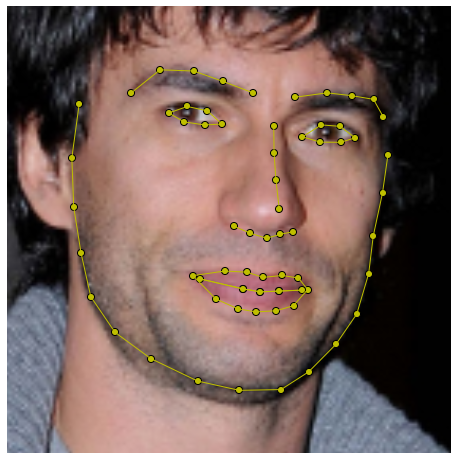


 A demonstration of the GamingAnywhere system. There are four devices in the photo. One game server (left-hand side labtop) and three game clients (an MacBook, an Android phone, and an iPad 2).


 Essentia is an open-source C++ library for audio analysis and audio-based music information retrieval released under the


